For the MFRU exhibition, we presented a variety of robots. The following is some documentation, on the specifications, and setup instructions. We are leaving the robots with konS.
All Robots
Li-Po batteries need to be stored at 3.8V per cell. For exhibition, they can be charged to 4.15A per cell, and run with a battery level monitor until they display 3.7V, at which point they should be swapped out. Future iterations of robotic projects will make use of splitter cables to allow hot swapping batteries, for zero downtime.
We leave our ISDT D2 Mark 2 charger, for maintaining and charging Li-Po batteries.
At setup time, in a new location, Raspberry Pi SD cards need to be updated to connect to the new Wi-fi network. Simplest method is to physically place the SD card in a laptop, and transfer a wpa_supplicant.conf file with the below changed to the new credentials and locale, and a blank file called ssh, to allow remote login.
Then following startup with the updated SD card, robot IP addresses need to be determined, typically using `nmap -sP 192.168.xxx.xxx`, (or a windows client like ZenMap).
Usernames and passwords used are:
LiDARbot – pi/raspberry
Vacuumbot – pi/raspberry and chicken/chicken
Pinkbot – pi/raspberry
Gripperbot – pi/raspberry
Birdbot – daniel/daniel
Nipplebot – just arduino
Lightswitchbot – just arduino and analog timer
For now, it is advised to shut down robots by connecting to their IP address, and typing sudo shutdown -H now and waiting for the lights to turn off, before unplugging. It’s not 100% necessary, but it reduces the chances that the apt cache becomes corrupted, and you need to reflash the SD card and start from scratch.
Starting from scratch involves reflashing the SD card using Raspberry Pi Imager, cloning the git repository, running pi_boot.sh and pip3 install -y requirements.txt, configuring config.py, and running create_service.sh to automate the startup.
LiDARbot
Raspberry Pi Zero W x 1 PCA9685 PWM controller x 1 RPLidar A1M8 x 1 FT5835M servo x 4
Powered by: Standard 5V Power bank [10Ah and 20Ah]
Startup Instructions: – Plug in USB cables. – Wait for service startup and go to URL. – If Lidar chart is displaying, click ‘Turn on Brain’
LiDARbot has a lidar, laser head spinning around, collecting distance updates from the light that bounces back, allowing it to update a 2d (top-down) map of its surroundings. It is able to not bump into things.
Vacuumbot
Raspberry Pi 3b x 1 LM2596 stepdown converter x 1 RDS60 servo x 4
Powered by: 7.4V 4Ah Li-Po battery
NVIDIA Jetson NX x 1 Realsense D455 depth camera x 1
Powered by: 11.1V 4Ah Li-Po battery
Instructions: – Plug Jetson assembly connector into 11.4V, and RPi assembly connector into 7.4V – Connect to Jetson:
cd ~/jetson-server
python3 inference_server.py
– Go to the Jetson URL to view depth and object detection. – Wait for Rpi service to start up. – Connect to RPi URL, and click ‘Turn on Brain’
It can scratch around, like the chickens.Vacuumbot has a depth camera, so it can update a 3d map of its surroundings, and it runs an object detection neural network, so it can interact with its environment. It uses 2 servos per leg, 1 for swivelling its hips in and out, and 1 for the leg rotation.
Pinkbot
Raspberry Pi Zero W x 1 PCA9685 PWM controller x 1 LM2596 stepdown converter x 1 RDS60 servo x 8 Ultrasonic sensors x 3
Powered by: 7.4V 6.8Ah Li-Po battery
Instructions: – Plug in to Li-Po battery – Wait for Rpi service to start up. – Connect to RPi URL, and click ‘Turn On Brain’
Pinkbot has 3 ultrasonic distance sensors, so it has a basic “left” “forward” “right” sense of its surroundings. It uses 8 x 60kg-cm servos, (2 per leg), and 2 x 35kg-cm servos for the head. The servos are powerful, so it can walk, and even jump around.
Gripperbot
Gripperbot has 4 x 60kg-cm servos and 1 x 35kg-cm continuous rotation servo with a worm gear, to open and close the gripper. It uses two spring switches which let it know when the hand is closed. A metal version would be cool.
Raspberry Pi Zero W x 1 150W stepdown converter (to 7.4V) x 1 LM2596 stepdown converter (to 5V) x 1 RDS60 servo x 4 MGGR996 servo x 1
Powered by: 12V 60W power supply
Instructions: – Plug in to wall – Wait for Rpi service to start up. – Connect to RPi URL, and click ‘Fidget to the Waves’
Birdbot
Raspberry Pi Zero W x 1 FT SM-85CL-C001 servo x 4 FE-URT-1 serial controller x 1 12V input step-down converter (to 5V) x 1 Ultrasonic sensor x 1 RPi camera v2.1 x 1
Powered by: 12V 60W power supply
Instructions: – Plug in to wall – Wait for Rpi service to start up. – Connect to RPi URL, and click ‘Fidget to the Waves’
Birdbot is based on the Max Planck Institute BirdBot, and uses some nice 12V servos. It has a camera and distance sensor, and can take pictures when chickens pass by. We didn’t implement the force sensor central pattern generator of the original paper, however. Each leg uses 5 strings held in tension, making it possible, with one servo moving the leg, and the other servo moving the string, to lift and place the leg with a more sophisticated, natural, birdlike motion.
I got the Feetech Smart Bus servos running on the RPi. Using them for the birdbot.
Some gotchas:
Need to wire TX to TX, RX to RX.
Despite claiming 1000000 baudrate, 115200 was required, or it says ‘There is no status packet!”
After only one servo working, for a while, I found their FAQ #5, and installed their debugging software, and plugged each servo in individually, and changed their IDs to 1/2/3/4. It was only running the first one because all of their IDs were still 1.
For python, you need to pip3 install pyserial, and then import serial.
I soldered on some extra wires to the motor + and -, to power the motor separately.
Wasn’t getting any luck, but it turned out to be the MicroUSB cable (The OTG cable was ok). After swapping it out, I was able to run the simple_grabber app and confirm that data was coming out.
I debugged the Adafruit v1.29 issue too. So now I’m able to get the data in python, which will probably be nicer to work with, as I haven’t done proper C++ in like 20 years. But this Slamtec code would be the cleanest example to work with.
So I added in some C socket code and recompiled, so now the demo app takes a TCP connection and starts dumping data.
It was actually A LOT faster than the python libraries. But I started getting ECONNREFUSED errors, which I thought might be because the Pi Zero W only has a single CPU, and the Python WSGI worker engine was eventlet, which only handles 1 worker, for flask-socketio, and running a socket server, client, and socket-io, on a single CPU, was creating some sort of resource contention. But I couldn’t solve it.
I found a C++ python-wrapped project but it was compiled for 64 bit, and the software, SWIG, which I needed to recompile for 32 bit, seemed a bit complicated.
So, back to Python.
Actually, back to javascript, to get some visuals in a browser. The Adafruit example is for pygame, but we’re over a network, so that won’t work. Rendering Matplotlib graphs is going to be too slow. Need to stream data, and render it on the front end.
Detour #1: NPM
Ok… so, need to install Node.js to install this one, which for Raspberry Pi Zero W, is ARM6.
This is the most recent ARM6 nodejs tarball:
wget https://nodejs.org/dist/latest-v11.x/node-v11.15.0-linux-armv6l.tar.gz

tar xzvf node-v11.15.0-linux-armv6l.tar.gz
cd node-v11.15.0-linux-armv6l
sudo cp -R * /usr/local/
sudo ldconfig
npm install --global yarn
sudo npm install --global yarn

npm install rplidar

npm ERR! serialport@4.0.1 install: `node-pre-gyp install --fallback-to-build`

Ok...  never mind javascript for now.
Detour #2: Dash/Plotly
Let’s try this python code. https://github.com/Hyun-je/pyrplidar
Ok well it looks like it works maybe, but where is s/he getting that nice plot from? Not in the code. I want the plot.
So, theta and distance are just polar coordinates. So I need to plot polar coordinates.
PolarToCartesian.
Convert a polar coordinate (r,θ) to cartesian (x,y): x = r cos(θ), y = r sin(θ)
pip3 install pandas
pip3 install dash

k let's try...
ValueError: numpy.ndarray size changed, may indicate binary incompatibility. Expected 48 from C header, got 40 from PyObject

ok
pip3 install --upgrade numpy
(if your numpy version is < 1.20.0)

ok now  bad marshal data (unknown type code)
sheesh, what garbage.
Posting issue to their github and going back to the plan.
Reply from Plotly devs: pip3 won’t work, will need to try conda install, for ARM6
Ok let’s see if we can install plotly again….
Going to try miniconda – they have a arm6 file here…
Damn. 2014. Python 2. Nope. Ok Plotly is not an option for RPi Zero W. I could swap to another RPi, but I don’t think the 1A output of the power bank can handle it, plus camera, plus lidar motor, and laser. (I am using the 2.1A output for the servos).
Solution #1: D3.js
Ok, Just noting this link, as it looks useful for the lidar robot, later.
“eventlet is the best performant option, with support for long-polling and WebSocket transports.”
apparently needs redis for message queueing…
pip install eventlet
pip install redis

Ok, and we need gunicorn, because eventlet is just for workers...

pip3 install gunicorn

gunicorn --worker-class eventlet -w 1 module:app

k, that throws an error.
I need to downgrade eventlet, or do some complicated thing.
pip install eventlet==0.30.2

gunicorn --bind 0.0.0.0 --worker-class eventlet -w 1 kmp8servo:app
(my service is called kmp8servo.py)


ok so do i need redis?
sudo apt-get install redis
ok it's already running now,
at /usr/bin/redis-server 127.0.0.1:6379
no, i don't really need redis.  Could use sqlite, too. But let's use it anyway.

Ok amazing, gunicorn works.  It's running on port 8000

Ok, after some work,  socket-io is also working.

Received #0: Connected
Received #1: I'm connected!
Received #2: Server generated event
Received #3: Server generated event
Received #4: Server generated event
Received #5: Server generated event
Received #6: Server generated event
Received #7: Server generated event
So, I’m going to go with d3.js instead of P5js, just cause it’s got a zillion more users, and there’s plenty of polar coordinate code to look at, too.
Got it drawing the polar background… but I gotta change the scale a bit. The code uses a linear scale from 0 to 1, so I need to get my distances down to something between 0 and 1. Also need radians, instead of the degrees that the lidar is putting out.
ok finally. what an ordeal.
But now we still need to get python lidar code working though, or switch back to the C socket code I got working.
Ok, well, so I added D3 update code with transitions, and the javascript looks great.
But the C Slamtec SDK, and the Python RP Lidar wrappers are a source of pain.
I had the C sockets working briefly, but it stopped working, seemingly while I added more Python code between each socket read. I got frustrated and gave up.
The Adafruit library, with the fixes I made, seem to work now, but it’s in a very precarious state, where looking at it funny causes a bad descriptor field, or checksum error.
But I managed to get the brain turning on, with the lidar. I’m using Redis to track the variables, using the memory.py code from this K9 repo. Thanks.
I will come back to trying to fix the remaining python library issues, but for now, the robot is running, so, on to the next.
This is turning into one of the most oddly complicated sub-tasks of making a robot.
Turns out you need an intuition for epipolar geometry, to understand what it’s trying to do.
I’ve been battling this for weeks or months, on-and-off, and I must get it working soon. This week. But I know a week won’t be enough. This shit is hairy. Here’s eleven tips on StackOverflow. And here’s twelve tips from another guru.
The only articles that look like they got it working, have printed out these A2 sized chessboards. It’s ridiculous. Children in Africa don’t have A2 sized chessboard printouts!
Side notes: I’d like to mention that there also seem to be some interesting developments, in the direction of not needing perfect gigantic chessboards to calibrate your cameras, which in turn led down a rabbit hole, into a galaxy of projects packaged together with their own robotics software philosophies, and so on. Specifically, I found this OpenHSML project. They packaged their project using PID framework. This apparently standardises the build process, in some way. Clicking on the links to officially released frameworks using PID, leads to RPC, ethercatcpp, hardio, RKCL, and a whole world of sensor fusion topics, including a recent IEEE conference on MultiSensor Fusion and Integration (MFI2021.org).
So, back to chessboards. It’s clearly more of an art than a science.
Let’s, for the sake of argument, use the code at this OpenCV URL on the topic.
Let’s fire up the engines. I really want to close some R&D tabs, but we’re down to about 30. I’ll try reduce, to 20, while we go through the journey, together, dear internet reader, or future intelligence. Step One. Install OpenCV. I’m using the ISAAC ROS common docker with various modifications. (Eg. installing matplotlib, Jupyter Lab)
cd ~/your_ws/src/isaac_ros_common

./scripts/run_dev.sh ~/your_ws/
python3
print(cv2.version) 4.5.0
So this version of the docs should work, surely. Let’s start up Jupyter because it looks like it wants it.
python3 example_1.py
example_1.py:61: UserWarning: Matplotlib is currently using agg, which is a non-GUI backend, so cannot show the figure.
plt.show()
Firing up Jupyter, inside the docker and check out http://chicken:8888/lab
admin@chicken:/workspaces$ jupyter lab --ip 0.0.0.0 --port 8888 --allow-root &

Let's run the code... let's work out how to make the images bigger, ok, plt.rcParams["figure.figsize"] = (30,20)
It’s definitely doing something. I see the epilines, they look the same. That looks great. Ok next tutorial.
So, StereoBM. “Depth Map from Stereo Images”
so, the top one is the disparity, viewed with StereoBM. Interesting. BM apparently means Block Matching. Interesting to see that the second run of the epiline code earlier, is changing behaviour. Different parallax estimation?
Changing the max disparities, and block size changes the image, kinda like playing with a photoshop filter. Anyway we’re here to calibrate. What next?
I think the winner for nicest website on the topic goes to Andreas Jakl here, professor.
“Here, we’ll use the traditional SIFT algorithm. Its patent expired in March 2020, and the algorithm got included in the main OpenCV implementation.”
Ok first things first, I’m tightening the screws into the camera holder plastic. We’re only doing this a few times.
Let’s run the capture program one more time for fun.
I edited the code to make the images 1280×720, which was one of the outputs of the camera. It’s apparently 16:9.
I took a bunch of left and right images. Ran it through the jetson-stereo-depth/calib/01_intrinsics_lens_dist.ipynb code, and the only chessboards it found were the smaller boards .
So let’s put back in the resizing. Yeah no. Ok. Got like 1 match out of 35.
Ok I’m giving up for now. But we’re printing, boys and girls. We’ll try A4 first, and see how it goes. Nope. A3. Professional print.
Nope. Nicely printed doesn’t matter.
Ran another 4 rounds of my own calibration code. Hundreds of pictures. You only need one match.
Nope. You can read more about messing around with failed calibration attempts in this section.
Asked NVIDIA – is it possible? Two monocular cameras into a stereo camera? – no reply. Two months later, NVIDIA replied. “problem will be time synchronizing their frames. You’ll also need to introduce the baseline into the camera_info of the right camera to make it work”
Time is running out. So I threw money at this problem.
Bought the Intel Realsense D455. At first glance, the programs that come with it are very cool, ‘realsense-viewer’. A bit freaky.
After checking out the speed of image segmentation on the Raspberry Pi (like one frame every 10 seconds maybe?), and my i3 laptop not being much better, I realised I needed more computing power, at least to train the neural networks. I can probably still ultimately run the neural network on the Pi, but we’ll see.
Looking at computing options, I ultimately went with the $399 NVIDIA Jetson Xavier NX.
Developer Kit Technical Specifications
GPU
NVIDIA Volta™ architecture with 384 NVIDIA® CUDA® cores and 48 Tensor cores
Gigabit Ethernet, M.2 Key E (WiFi/BT included), M.2 Key M (NVMe)
Display
HDMI and DP
USB
4x USB 3.1, USB 2.0 Micro-B
Others
GPIOs, I2C, I2S, SPI, UART
Mechanical
103 mm x 90.5 mm x 34 mm
Also, did you know they made a dystopic reboot retcon of The Jetsons, that 70s retro-futuristic Hanna Barbera cartoon, in comic form? An ice meteor destoyed Earth. They were lucky to have had a place in space to go, working for the Spacely Space Sprockets, incorporated. (YT link)
It took an hour to set up, and was mostly straightforward, though I had to get a ‘clover plug’ cable, and an SD card.
I used Etcher to load the latest 6GB Jetson Developer Kit SD image, and had a keyboard, mouse, and hdmi monitor that worked. So I was able to enter the wifi SSID and password while setting it up.
I learned that one option for headless installation is to use a USB cable from your computer to the micro-USB input of the Jetson. But ultimately this wasn’t necessary. I ran ipconfig on the Jetson, got an ip address, and connected with ssh.
After needing to change the wifi details, I used the usb cable, then connected with:
Coming back to this later, I attempted the same, but with the Jetson Nano, instead of the Jetson Xavier, and it didn’t work. I learned that the Nano doesn’t come with a Wifi adapter.
I think with the Nano, (“B01”) you need a monitor to install. I tried multiple tutorials, ssh’ing 192.168.55.1, I tried using screen to connect to /dev/ttyACC0 at 115200 baud, nope. Looked at the forums, and it’s complicated. I didn’t try the USB UART because my USB-TTL converter’s cable colours are different.
Another method that worked, with the nano, is plugging the ethernet cable from the Nano directly into the wifi router. It then shows up on the router’s network.
Later, when trying to install a D-Link wifi ‘Wireless N Nano USB Adaptor’, ( for the love of God, just get an Edimax – they work out of the box), I connected over ssh with the ethernet cable from the jetson to the router, then downloaded the driver and unzipped and untarred, and then ran the `make` file and `make install` as per the instructions, but had to run export ARCH=arm64 before that, because it was looking in aarch64. Then rebooted. Then
chicken@chicken:~$ sudo nmcli device wifi connect 'ssid' password 'password'
[sudo] password for chicken:
Device 'wlan0' successfully activated with '3a7997e6-c6b1-40f7-bf93-fba5b110282c'.
A lot of research will have to happen again now, though, because NVIDIA has its own software ecosystem. I’ll need a vision solution that is portable to the PI, with the hope that a model or neural net trained on the Jetson will still be able to run on the Raspberry Pi, since it’s 40X cheaper.
The lingo takes some time to get used to, but I believe JetPack is the name for this OS of preinstalled nvidia docs and libraries.
Since last year, an algorithm called… a Transformer… which has just recently created a hell of a chat bot, with GPT-3, and which underlies Google search as BERT (Bidirectional Encoder Representations from Transformers).
And there are hybrid convolutional nets and transformers, eg. DETR, and there are the SOTA from last year, EfficientNet, and then for some instances, or most, YOLOv4 is meant to be the new hot algorithm. It’s bigger than YOLOv3. It’s wait, so it’s more frames per second, and the accuracy (AP) is kinda so/so, at 5% less. I realised YOLOv5, which I had seen, which is a Pytorch implementation, is faster, though it’s technically just some one being a bit of a douchebag and calling his implementation of the author’s peer reviewed, the next version, YOLOv5. So what now?
NVIDIA has this 3d simulator environment in Unreal Engine! Isaac. Something like an API for robots, by NVIDIA. They got this robot working with it, apparently.
It’s actually pretty good. I wonder if this https://developer.nvidia.com/deepstream-sdk is as cool as it sounds. Ah, closed source. Of course. But I can apply to join. Eh maybe.
So, I want to get these chickens into a convolutional neural network, or a transformer and output a pretty picture. I want the colour masks, not the bounding boxes.
I don’t want to get too caught up in proprietary NVIDIA specific API, even if they have an Unreal Engine simulator. But it might be worth checking out. GStreamer is an open source port of it, so maybe back on the menu.
But it’s a whole integrated thing. “The DeepStream SDK can be used to build end-to-end AI-powered applications to analyze video and sensor data. Some popular use cases are: retail analytics, parking management, managing logistics, robotics, optical inspection and managing operations.”
Nice. DeepStream supports several popular networks out of the box such as YOLO, FasterRCNN, SSD, RetinaNet and MaskRCNN.
I get the sense that Gems in the DeepStream world of Isaac, are like, ROS nodes, offering services on a port. ORB is a Gem. Ultimately, a prediction, or reconstruction in 3d, of the shape of objects in the world, would be ideal. I’m only doing the colour map stuff because the colours are nice, and it looks more impressive. But ultimately I will need to pick the best tool for the job.
NVIDIA also has DIGITS, Deep Learning GPU Training System (DIGITS) … puts the power of deep learning into the hands of engineers and data scientists. DIGITS can be used to rapidly train the highly accurate deep neural network (DNNs) for image classification, segmentation and object detection tasks.
So as you can see, there’s more to find out. But ultimately I will probably have to repeat the task of getting labelled data into folders, and having the labels in the right format. Then generating the TFRecords, or doing whatever you do in PyTorch, I’m still biased to the TensorFlow ODI 2 implementation, because Google’s got the best dataset of chickens.
We should check out rotary encoders and motors, while I’m in RSA. I’ve started looking at them now. There’s a wealth of info at a company that makes them, Dynapar.
Here’s the good stuff. Coupling: “Rotary encoders come in 3 major mounting styles: hollow-shaft (hollow-bore or through shaft), hub-shaft (hub-bore) or shafted. Hollow-shaft and hub-shaft rotary encoders mount directly to a motor shaft typically using a tether. Shafted rotary encoders mount using a flexible coupling.”
I asked a South African company about their Italian ‘Eltra‘ rotary encoders yesterday. Then Feetech from China asked this morning, if I needed servos. Well actually yes. I asked about their encoder motors, as they might be called, as a combination. They had 4.8V, 6V, and 7.4V such motors, whose encoders were of the magnetic measuring type, and give 12 bits of precision (2^12 = 4096, so 0 to 4095) as serial data.
The MG996Rs used for the basic table robot prototype were possibly adequate, but definitely on the hobby side. They felt more appropriate for a robot about half the size of the prototype. The prototype was successfully sat upon, by the chicken.
I started thinking about practicalities of powering a jetson nx (The devkit supports between 9-20V ) or jetson nano (5V) ot rpi (5V). and numerous motors. So probably uses a battery in the 9-20V range. Motor too. Probably 14.4V is what Lithium ion or similar batteries come as. Usually need to buy lithium ion batteries in the place where you’re going, rather than bring them on a plane. But you can always try. (Not a financial advisor (or otherwise)). They are probably still mostly imported for RC models (remote control, remember?).
Used his own interesting and as yet mysterious encoder, which he put inside a motor. Says his robot arm cost EU 300. It’s super impressive.
The other option with power appears to be cool ‘just what you needed’ type products like DFRobot’s FIT0186, which has a built-in encoder! I ended up buying 4 x FIT0186s and 4 x FIT0185s (12V, 251RPM and 83RPM respectively).
I used an Arduino Nano, a DFRobot Dual motor driver, based on the TB6612 chip, plugging in the Nano for 5V, and 12V into the driver, to power the motors.
But after much wiring up, the motors work fine, but the encoders do not. I fixed up their example code to use volatile variables, and run the minimal amount of code in the interrupt service routines (ISRs), and even used two interrupts for a single motor, one for each hall sensor output, and put a 0.1mF capacitor between signal and ground. Tried CHANGE/RISING/FALLING triggers. Tried different motors.
I’ve looked at every forum post, and tried everything, and now I’ve posted on DFRobot’s forum, in case someone has got the encoder working. Not looking promising.
So back to the MG996Rs, I find that I ordered two batches from Mantech, supposedly the same genuine product from Tower Pro, and yet the one batch does not work properly with the PCA9685, uses a lower minimum pulse, and moves in the opposite direction to the other ones when using the same code. The duds keep creeping around, after you turn off the throttle.
Ok so I’m going to try with the one batch of MG996Rs that do seem to work, but we’ll need to make a new plan. Possibly, rigging an actual rotary encoder up, on the motor shaft. But for now, back to MG996Rs and the drawing board. We left the old robotable in Switzerland last year. So I made a new one with the remaining MG996Rs.
So I was able to get them fairly well calibrated by setting the min and max pulse, as that seems to be how servos work. They have a center PWM pulse, around 1500, where they are still, and then as you decrease the pulses per second, it goes one way, and as you increase the pulses per second, it goes the other way.
Unfortunately after much fuss, these continuous rotation servos turned out to be duds. At least for the way I was trying to use them.
Set the throttle to 1, sleep for a second. Set the throttle to zero, sleep for a second. Set the throttle to -1, sleep for a second. …And you have a new position. Unfortunately the positional control is unusable. I guess these are for wheels or an application where position is not so important.
Months have passed. It is 29 December 2020 now, and Miranda and I are at Bitwäscherei, in Zurich, during the remoteC3 (Chaos Computer Club)
We have a few things to get back to:
Locomotion
Sim2Real
Vision
Object detection / segmentation
We plan to work on a chicken cam, but are waiting for the raspberry pi camera to arrive. So first, locomotion.
Miranda would like to add more leg segments, but process-wise, we need the software and hardware working together with basics, before adding more parts.
Sentient Table prototype
I’ve tested the GPIO, and it’s working, after adjusting the minimum pulse value for the MG996R servo.
So, where did we leave off, before KonS MFRU / ICAF ?
Locomotion:
There was a walking table in simulation, and the progress was saving so that we could reload the state, in Ray and Tune.
I remember the best walker had a ‘reward’ of 902, so I searched for 902
grep -R ‘episode_reward_mean\”\: 902’
And found these files:
 409982 Aug 1 07:52 events.out.tfevents.1596233543.chrx
 334 Jul 31 22:12 params.json
 304 Jul 31 22:12 params.pkl
 132621 Aug 1 07:52 progress.csv
 1542332 Aug 1 07:52 result.json
and there are checkpoint directories, with binary files.
So what are these files? How do I extract actions?
Well it looks like this info keeps track of Ray/Tune progress. If we want logs, we seem to need to make them ourselves. The original minitaur code used google protobuf to log state. So I set the parameter to log to a directory.
log_path="/media/chrx/0FEC49A4317DA4DA/logs"
So now when I run it again, it makes a file in the format below:
message RobotableEpisode {
  // The state-action pair at each step of the log.
  repeated RobotableStateAction state_action = 1;
}

message RobotableMotorState {
  // The current angle of the motor.
  double angle = 1;
  // The current velocity of the motor.
  double velocity = 2;
  // The current torque exerted at this motor.
  double torque = 3;
  // The action directed to this motor. The action is the desired motor angle.
  double action = 4;
}

message RobotableStateAction {
  // Whether the state/action information is valid. It is always true if the
  // proto is from simulation. It might be false when communication error
  // happens on robotable hardware.
  bool info_valid = 6;
  // The time stamp of this step. It is computed since the reset of the
  // environment.
  google.protobuf.Timestamp time = 1;
  // The position of the base of the minitaur.
  robotics.messages.Vector3d base_position = 2;
  // The orientation of the base of the minitaur. It is represented as (roll,
  // pitch, yaw).
  robotics.messages.Vector3d base_orientation = 3;
  // The angular velocity of the base of the minitaur. It is the time derivative
  // of (roll, pitch, yaw).
  robotics.messages.Vector3d base_angular_vel = 4;
  // The motor states (angle, velocity, torque, action) of eight motors.
  repeated RobotableMotorState motor_states = 5;
}
I’m pretty much only interested in that last line,
repeated RobotableMotorState motor_states = 5;
So that’s the task, to decode the protobuf objects.
import os
import inspect

currentdir = os.path.dirname(os.path.abspath(inspect.getfile(inspect.currentframe())))
parentdir = os.path.dirname(os.path.dirname(currentdir))
os.sys.path.insert(0, parentdir)

import argparse
from gym_robotable.envs import logging

if __name__ == "__main__":

    parser = argparse.ArgumentParser(formatter_class=argparse.ArgumentDefaultsHelpFormatter)
    parser.add_argument('--log_file', help='path to protobuf file', default='/media/chrx/0FEC49A4317DA4DA/logs/robotable_log_2020-12-29-191602')
    args = parser.parse_args()
    logging = logging.RobotableLogging()
    episode = logging.restore_episode(args.log_file)
    print(dir (episode))
    print("episode=",episode)
    fields = episode.ListFields()

    for field in fields:
        print(field)
This prints out some json-like info. On the right path.
I decided to use StreamLit, which is integrated with various plotting libraries. After looking at the different plotting options, Plotly seems the most advanced.
Plotly uses Panda dataframes, which is tabular data. 2 dimensions. So I need to transform this to something usable.
Something like time on the x-axis
and angle / velocity / torque / action on the y axis.
Ok so how to do this…?
Well I’ve almost got it, but I mostly had to give up on StreamLit’s native line_chart for now. Plotly’s has line chart code that can handle multiple variables. So I’m getting sidetracked by this bug:
When I import plotly’s library,
import plotly.graph_objects as go
“No module named ‘plotly.graph_objects’; ‘plotly’ is not a package”
“This is the well known name shadowing trap.” – stackoverflow
I named my file plotly.py – that is the issue.
So, ok run it again… (streamlit run plot.py) and open localhost:8501…
Now,
Running as root without --no-sandbox is not supported. See https://crbug.com/638180
Ah ha. I went back to StreamLit notation and it worked.
#fig.show()
st.plotly_chart(fig)
Ok excellent, so here is my first round of code:
import pandas as pd
import numpy as np
import streamlit as st
import time
from plotly import graph_objects as go
import os
import inspect
from google.protobuf.json_format import MessageToJson
import argparse
from gym_robotable.envs import logging


currentdir = os.path.dirname(os.path.abspath(inspect.getfile(inspect.currentframe())))
parentdir = os.path.dirname(os.path.dirname(currentdir))
os.sys.path.insert(0, parentdir)


if __name__ == "__main__":


    st.title('Analyticz')


    parser = argparse.ArgumentParser(formatter_class=argparse.ArgumentDefaultsHelpFormatter)
    parser.add_argument('--log_file', help='path to protobuf file', default='/media/chrx/0FEC49A4317DA4DA/logs/robotable_log_2020-12-29-191602')
    args = parser.parse_args()
    logging = logging.RobotableLogging()
    episode_proto = logging.restore_episode(args.log_file)


    times = []
    angles = [[]]*4           # < bugs!
    velocities = [[]]*4
    torques = [[]]*4
    actions = [[]]*4

    for step in range(len(episode_proto.state_action)):

       step_log = episode_proto.state_action[step]
       times.append(str(step_log.time.seconds) + '.' + str(step_log.time.nanos))

       for i in range(4):
           angles[i].append(step_log.motor_states[i].angle)
           velocities[i].append(step_log.motor_states[i].velocity)
           torques[i].append(step_log.motor_states[i].torque)
           actions[i].append(step_log.motor_states[i].action)

    print(angles)
    print(times)
    print(len(angles))
    print(len(velocities))
    print(len(torques))
    print(len(actions))
    print(len(times))

    # Create traces
    fig = go.Figure()
    fig.add_trace(go.Scatter(x=times, y=angles[0],
	            mode='lines',
	            name='Angles'))
    fig.add_trace(go.Scatter(x=times, y=velocities[0],
	            mode='lines+markers',
	            name='Velocities'))
    fig.add_trace(go.Scatter(x=times, y=torques[0],
	            mode='markers',
                    name='Torques'))
    fig.add_trace(go.Scatter(x=times, y=actions[0],
	            mode='markers',
                    name='Actions'))

    st.plotly_chart(fig)
And it’s plotting data for one leg.
If this is just 5 seconds of simulation, then velocities looks like it might be the closest match. You can imagine it going up a bit, back a bit, then a big step forward.
So, one idea is to do symbolic regression, to approximate the trigonometry equations for quadrupedal walking, (or just google them), and generalise to a walking algorithm, to use for locomotion. I could use genetic programming, like at university (https://gplearn.readthedocs.io/en/stable/examples.html#symbolic-regressor). But that’s overkill and probably won’t work. Gotta smooth the graph incrementally. Normalize it.
Let’s see what happens next, visually, after 5 seconds of data, and then view the same, for other legs.
Ok there is 30 seconds of walking.
The tools I wrote for the walker, are run with ‘python3 play_tune.py –replay 1’. It looks for the best checkpoint and replays it from there.
But now I seem to be getting the same graph for different legs. What? We’re going to have to investigate.
Ok turns out [[]]*4 is the wrong way to initialise arrays in python. It makes all sublists the same. Here’s the correct way:
velocities = [[] for i in range(4)]
Now I have 4 different legs.
The graph is very spiky, so I’ve added a rolling window average, and normalised it between -1 and 1 since that’s what the servo throttle allows.
I am thinking that maybe because the range between min and max for the 4 legs are:
The rear legs aren’t moving as much, so maybe it doesn’t make sense to normalize them all to [-1, 1] all on the same scale. Like maybe the back right leg that moves so much should be normalized to [-1, 1] and then all the other legs are scaled down proportionally. Anyway, let’s see. Good enough for now.
In the code, the motors order is:
front right, front left, back right, back left.
Ok so to save the outputs…
import pandas as pd
 import numpy as np
 import streamlit as st
 import time
 from plotly import graph_objects as go
 import os
 import inspect
 from google.protobuf.json_format import MessageToJson
 import argparse
 from gym_robotable.envs import logging
 import plotly.express as px
 currentdir = os.path.dirname(os.path.abspath(inspect.getfile(inspect.currentframe())))
 parentdir = os.path.dirname(os.path.dirname(currentdir))
 os.sys.path.insert(0, parentdir)
 def normalize_negative_one(img):
     normalized_input = (img - np.amin(img)) / (np.amax(img) - np.amin(img))
     return 2*normalized_input - 1
 if name == "main":
     st.title('Analyticz')
     parser = argparse.ArgumentParser(formatter_class=argparse.ArgumentDefaultsHelpFormatter)
     parser.add_argument('--log_file', help='path to protobuf file', default='/media/chrx/0FEC49A4317DA4DA/walkinglogs/robotable_log_2021-01-17-231240')
     args = parser.parse_args()
     logging = logging.RobotableLogging()
     episode_proto = logging.restore_episode(args.log_file)
     times = []
     velocities = [[] for i in range(4)]
     for step in range(len(episode_proto.state_action)):
        step_log = episode_proto.state_action[step]
        times.append(str(step_log.time.seconds) + '.' + str(step_log.time.nanos))
        for i in range(4):
            velocities[i].append(step_log.motor_states[i].velocity)
     #truncate because a bunch of trailing zeros
     velocities[0] = velocities[0][0:3000]
     velocities[1] = velocities[1][0:3000]
     velocities[2] = velocities[2][0:3000]
     velocities[3] = velocities[3][0:3000]
     times = times[0:3000]
     #get moving averages
     window_size_0=40
     numbers_series_0 = pd.Series(velocities[0])
     windows_0 = numbers_series_0.rolling(window_size_0)
     moving_averages_0 = windows_0.mean()
     moving_averages_list_0 = moving_averages_0.tolist()
     without_nans_0 = moving_averages_list_0[window_size_0 - 1:]
     window_size_1=40
     numbers_series_1 = pd.Series(velocities[1])
     windows_1 = numbers_series_1.rolling(window_size_1)
     moving_averages_1 = windows_1.mean()
     moving_averages_list_1 = moving_averages_1.tolist()
     without_nans_1 = moving_averages_list_1[window_size_1 - 1:]
     window_size_2=40
     numbers_series_2 = pd.Series(velocities[2])
     windows_2 = numbers_series_2.rolling(window_size_2)
     moving_averages_2 = windows_2.mean()
     moving_averages_list_2 = moving_averages_2.tolist()
     without_nans_2 = moving_averages_list_2[window_size_2 - 1:]
     window_size_3=40
     numbers_series_3 = pd.Series(velocities[3])
     windows_3 = numbers_series_3.rolling(window_size_3)
     moving_averages_3 = windows_3.mean()
     moving_averages_list_3 = moving_averages_3.tolist()
     without_nans_3 = moving_averages_list_3[window_size_3 - 1:]
     #normalize between -1 and 1
     avg_0 = np.asarray(without_nans_0)
     avg_1 = np.asarray(without_nans_1)
     avg_2 = np.asarray(without_nans_2)
     avg_3 = np.asarray(without_nans_3)
     avg_0 = normalize_negative_one(avg_0)
     avg_1 = normalize_negative_one(avg_1)
     avg_2 = normalize_negative_one(avg_2)
     avg_3 = normalize_negative_one(avg_3)
     np.save('velocity_front_right', avg_0)
     np.save('velocity_front_left', avg_1)
     np.save('velocity_back_right', avg_2)
     np.save('velocity_back_left', avg_3)
     np.save('times', times)
     # Create traces
     fig0 = go.Figure()
     fig0.add_trace(go.Scatter(x=times, y=velocities[0],
                 mode='lines',
                 name='Velocities 0'))
     fig0.add_trace(go.Scatter(x=times, y=avg_0.tolist(),
                 mode='lines',
                 name='Norm Moving Average 0'))
     st.plotly_chart(fig0)
     fig1 = go.Figure()
     fig1.add_trace(go.Scatter(x=times, y=velocities[1],
                 mode='lines',
                 name='Velocities 1'))
     fig1.add_trace(go.Scatter(x=times, y=avg_1.tolist(),
                 mode='lines',
                 name='Norm Moving Average 1'))
     st.plotly_chart(fig1)
     fig2 = go.Figure()
     fig2.add_trace(go.Scatter(x=times, y=velocities[2],
                 mode='lines',
                 name='Velocities 2'))
     fig2.add_trace(go.Scatter(x=times, y=avg_2.tolist(),
                 mode='lines',
                 name='Norm Moving Average 2'))
     st.plotly_chart(fig2)
     fig3 = go.Figure()
     fig3.add_trace(go.Scatter(x=times, y=velocities[3],
                 mode='lines',
                 name='Velocities 3'))
     fig3.add_trace(go.Scatter(x=times, y=avg_3.tolist(),
                 mode='lines',
                 name='Norm Moving Average 3'))
     st.plotly_chart(fig3)
(Excuse the formatting.) Then I’m loading those npy files and iterating them to the motors.
So, it’s not terrible, but we’re not quite there either. Also i think it’s walking backwards.
I am not sure the math is correct.
I changed the smoothing code to use this code which smoothes based on the preceding plot.
def anchor(signal, weight):
     buffer = []
     last = signal[0]
     for i in signal:
         smoothed_val = last * weight + (1 - weight) * i
         buffer.append(smoothed_val)
         last = smoothed_val
     return buffer
Derp.
OK i realised I was wrong all along. Two things.
First, I just didn’t see that the angles values were on that original graph. They were so small. Of course we’re supposed to use the angles, rather than the velocities, for 180 degree servos.
Second problem was, I was normalizing from min to max of the graph. Of course it should be -PI/2 to PI/2, since the simulator works with radians, obviously. Well anyway, hindsight is 20/20. Now we have a fairly accurate sim2real. I use the anchor code above twice, to get a really smooth line.
Here’s the final code.
import pandas as pd
 import numpy as np
 import streamlit as st
 import time
 from plotly import graph_objects as go
 import os
 import inspect
 from google.protobuf.json_format import MessageToJson
 import argparse
 from gym_robotable.envs import logging
 import plotly.express as px
 currentdir = os.path.dirname(os.path.abspath(inspect.getfile(inspect.currentframe())))
 parentdir = os.path.dirname(os.path.dirname(currentdir))
 os.sys.path.insert(0, parentdir)
 def anchor(signal, weight):
     buffer = []
     last = signal[0]
     for i in signal:
         smoothed_val = last * weight + (1 - weight) * i
         buffer.append(smoothed_val)
         last = smoothed_val
     return buffer
 assume radians
 def normalize_0_180(img):
     normalized_0_180 = np.array(img)*57.2958 + 90
     return normalized_0_180
 if name == "main":
     st.title('Analyticz')
     parser = argparse.ArgumentParser(formatter_class=argparse.ArgumentDefaultsHelpFormatter)
     parser.add_argument('--log_file', help='path to protobuf file', default='/media/chrx/0FEC49A4317DA4DA/walkinglogs/robotable_log_2021-01-17-231240')
     args = parser.parse_args()
     logging = logging.RobotableLogging()
     episode_proto = logging.restore_episode(args.log_file)
     times = []
     angles = [[] for i in range(4)]
     for step in range(len(episode_proto.state_action)):
        step_log = episode_proto.state_action[step]
        times.append(str(step_log.time.seconds) + '.' + str(step_log.time.nanos))
        for i in range(4):
            print (step)
            print (step_log.motor_states[i].angle)
            angles[i].append(step_log.motor_states[i].angle)
     #truncate because a bunch of trailing zeros
     angles[0] = angles[0][0:3000]
     angles[1] = angles[1][0:3000]
     angles[2] = angles[2][0:3000]
     angles[3] = angles[3][0:3000]
     avg_0 = normalize_0_180(angles[0])
     avg_1 = normalize_0_180(angles[1])
     avg_2 = normalize_0_180(angles[2])
     avg_3 = normalize_0_180(angles[3])
     avg_0 = anchor(avg_0, 0.8)
     avg_1 = anchor(avg_1, 0.8)
     avg_2 = anchor(avg_2, 0.8)
     avg_3 = anchor(avg_3, 0.8)
     avg_0 = anchor(avg_0, 0.8)
     avg_1 = anchor(avg_1, 0.8)
     avg_2 = anchor(avg_2, 0.8)
     avg_3 = anchor(avg_3, 0.8)
     avg_0 = anchor(avg_0, 0.8)
     avg_1 = anchor(avg_1, 0.8)
     avg_2 = anchor(avg_2, 0.8)
     avg_3 = anchor(avg_3, 0.8)
     np.save('angle_front_right_180', avg_0)
     np.save('angle_front_left_180', avg_1)
     np.save('angle_back_right_180', avg_2)
     np.save('angle_back_left_180', avg_3)
     # Create traces
     fig0 = go.Figure()
     fig0.add_trace(go.Scatter(x=times, y=angles[0],
                 mode='lines',
                 name='Angles 0'))
     fig0.add_trace(go.Scatter(x=times, y=avg_0,
                  mode='lines',
                  name='Norm Moving Average 0'))
     st.plotly_chart(fig0)
     fig1 = go.Figure()
     fig1.add_trace(go.Scatter(x=times, y=angles[1],
                 mode='lines',
                 name='Angles 1'))
     fig1.add_trace(go.Scatter(x=times, y=avg_1,
                  mode='lines',
                  name='Norm Moving Average 1'))
     st.plotly_chart(fig1)
     fig2 = go.Figure()
     fig2.add_trace(go.Scatter(x=times, y=angles[2],
                 mode='lines',
                 name='Angles 2'))
     fig2.add_trace(go.Scatter(x=times, y=avg_2,
                  mode='lines',
                  name='Norm Moving Average 2'))
     st.plotly_chart(fig2)
     fig3 = go.Figure()
     fig3.add_trace(go.Scatter(x=times, y=angles[3],
                 mode='lines',
                 name='Angles 3'))
     fig3.add_trace(go.Scatter(x=times, y=avg_3,
                  mode='lines',
                  name='Norm Moving Average 3'))
     st.plotly_chart(fig3)
OK.
So there’s a milestone that took way too long. We’ve got Sim 2 Real working, ostensibly.
After some fortuitous googling, I found the Spot Micro, or, Spot Mini Mini project. The Spot Micro guys still have a big focus on inverse kinematics, which I’m trying to avoid for as long as I can.
They’ve done a very similar locomotion project using pyBullet, and I was able to find a useful paper, in the inspiration section, alerting me to kMPs.
Instead, what these guys did was to take a single wave of their leg data, and repeat that, and compare that to a standardized phase. (More or less). Makes sense. Looks a bit complicated to work out the phase of the wave in my case.
I’ll make a new topic, and try to extract kMPs from the data, for the next round of locomotion sim2real. I will probably also train the robot for longer, to try evolve a gait that isn’t so silly.
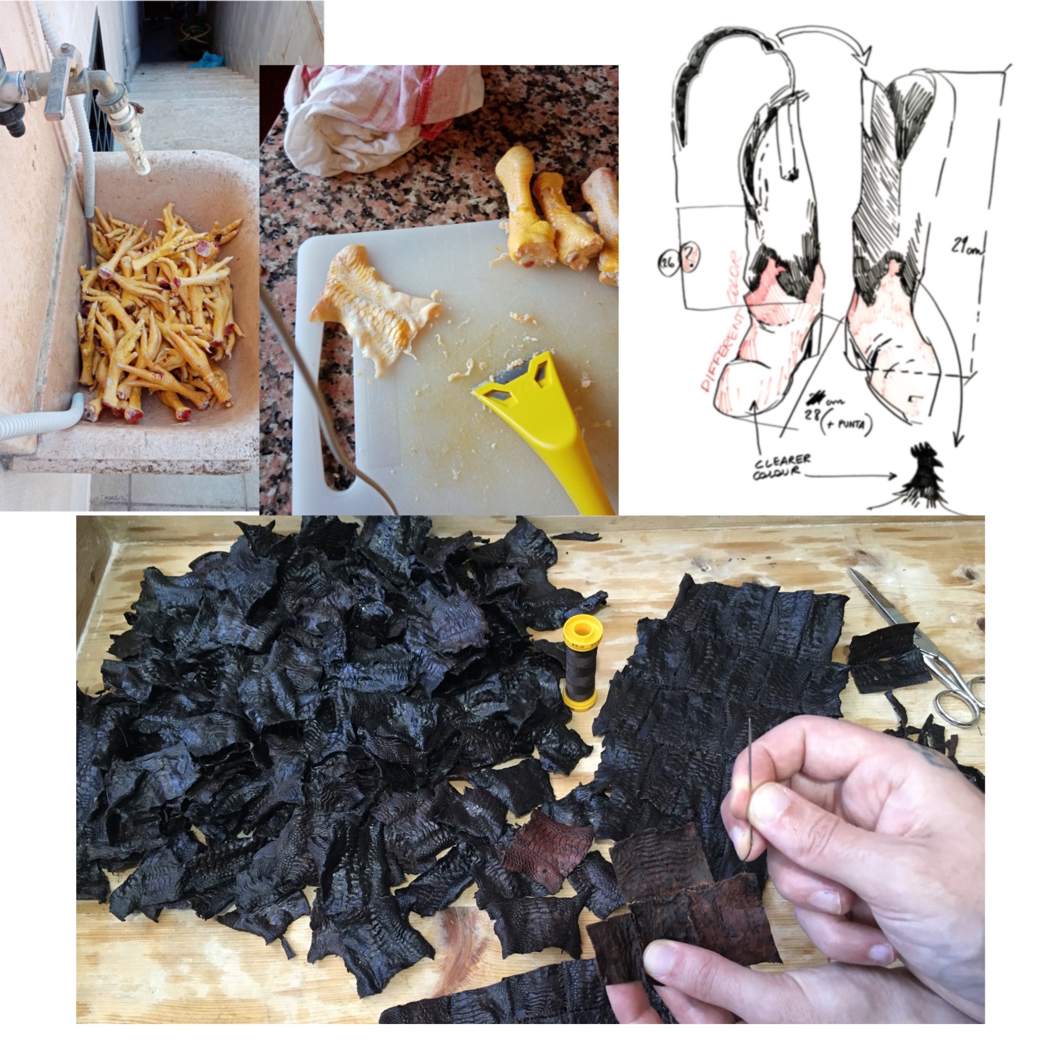
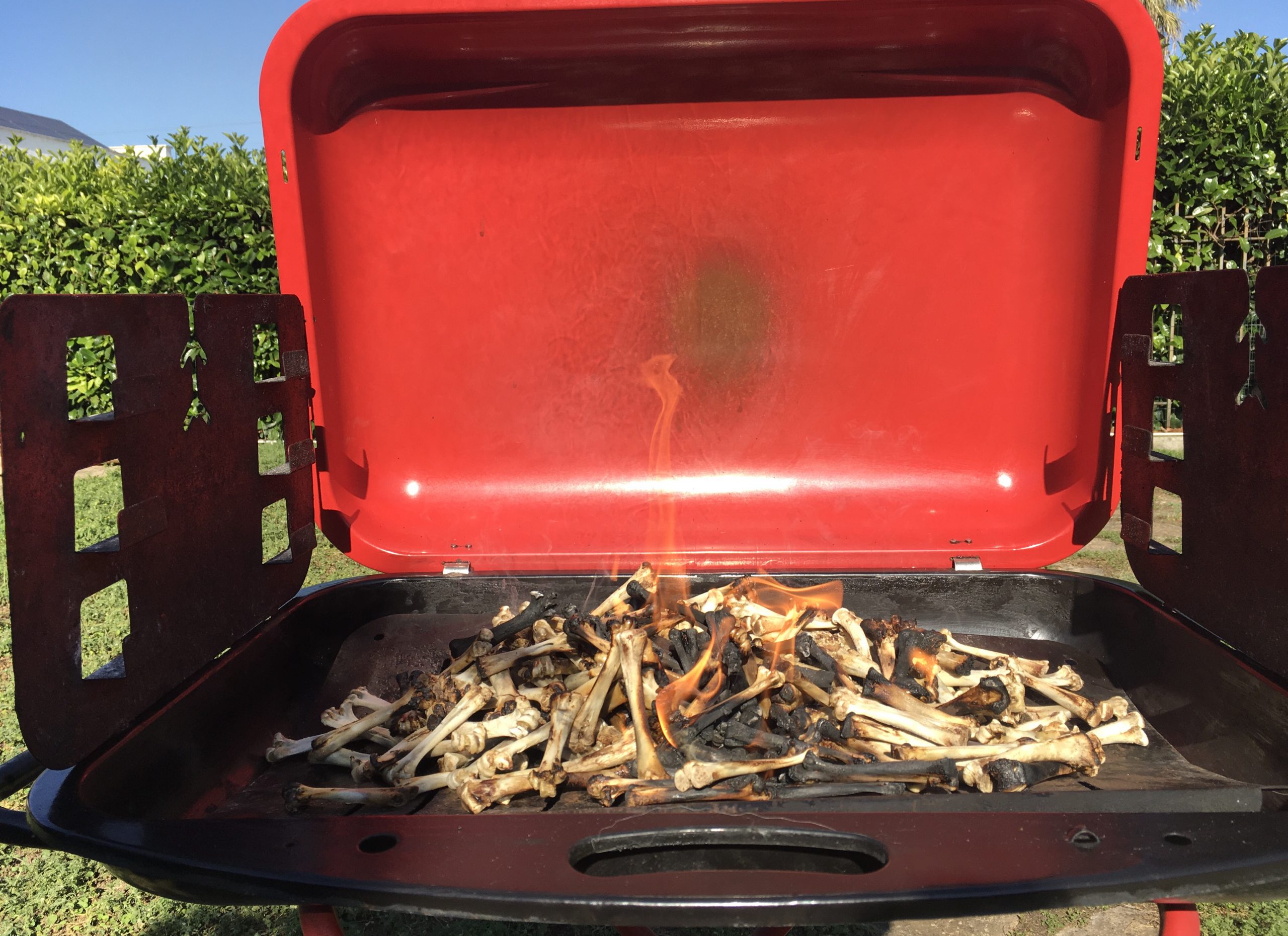
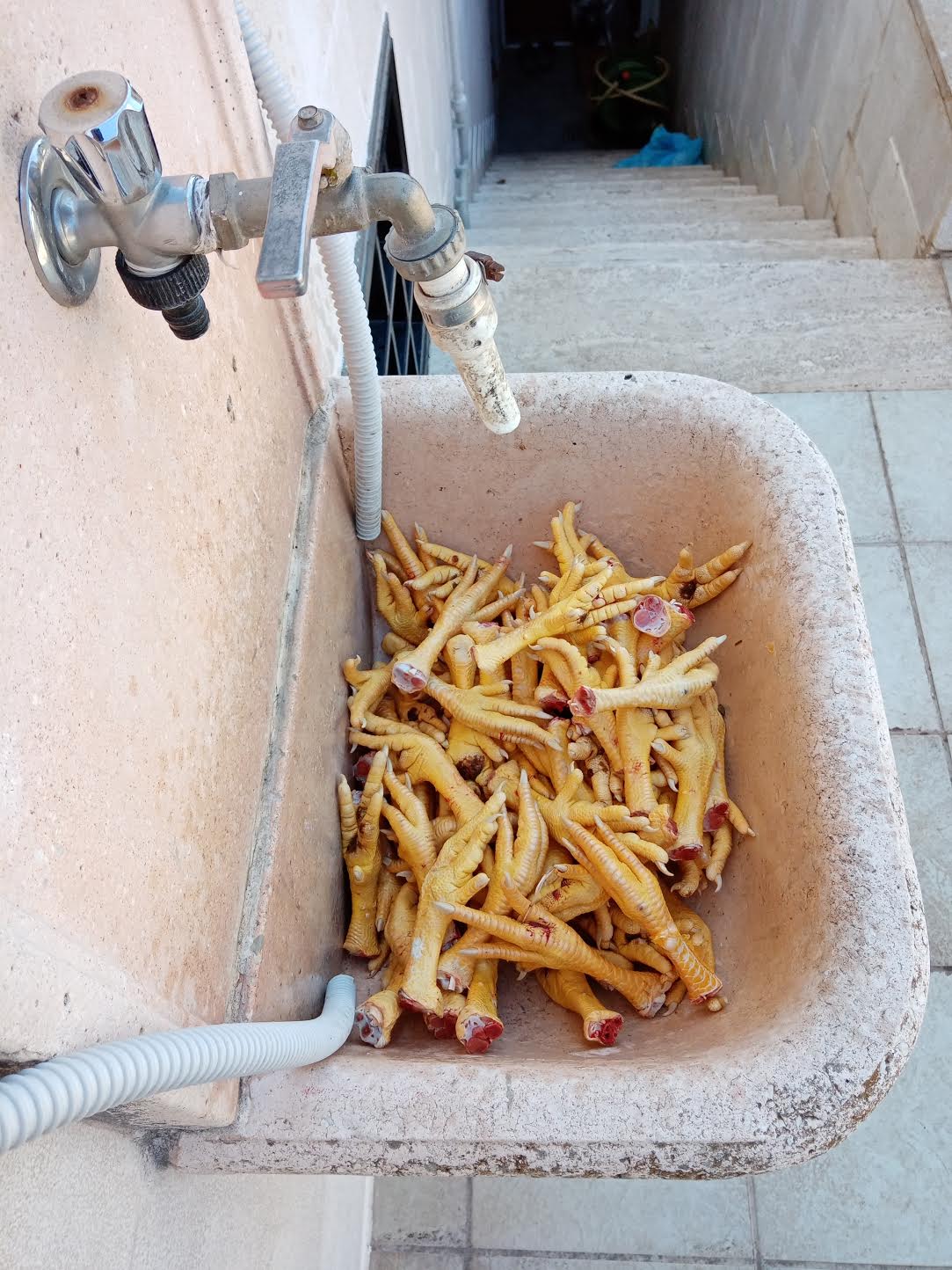
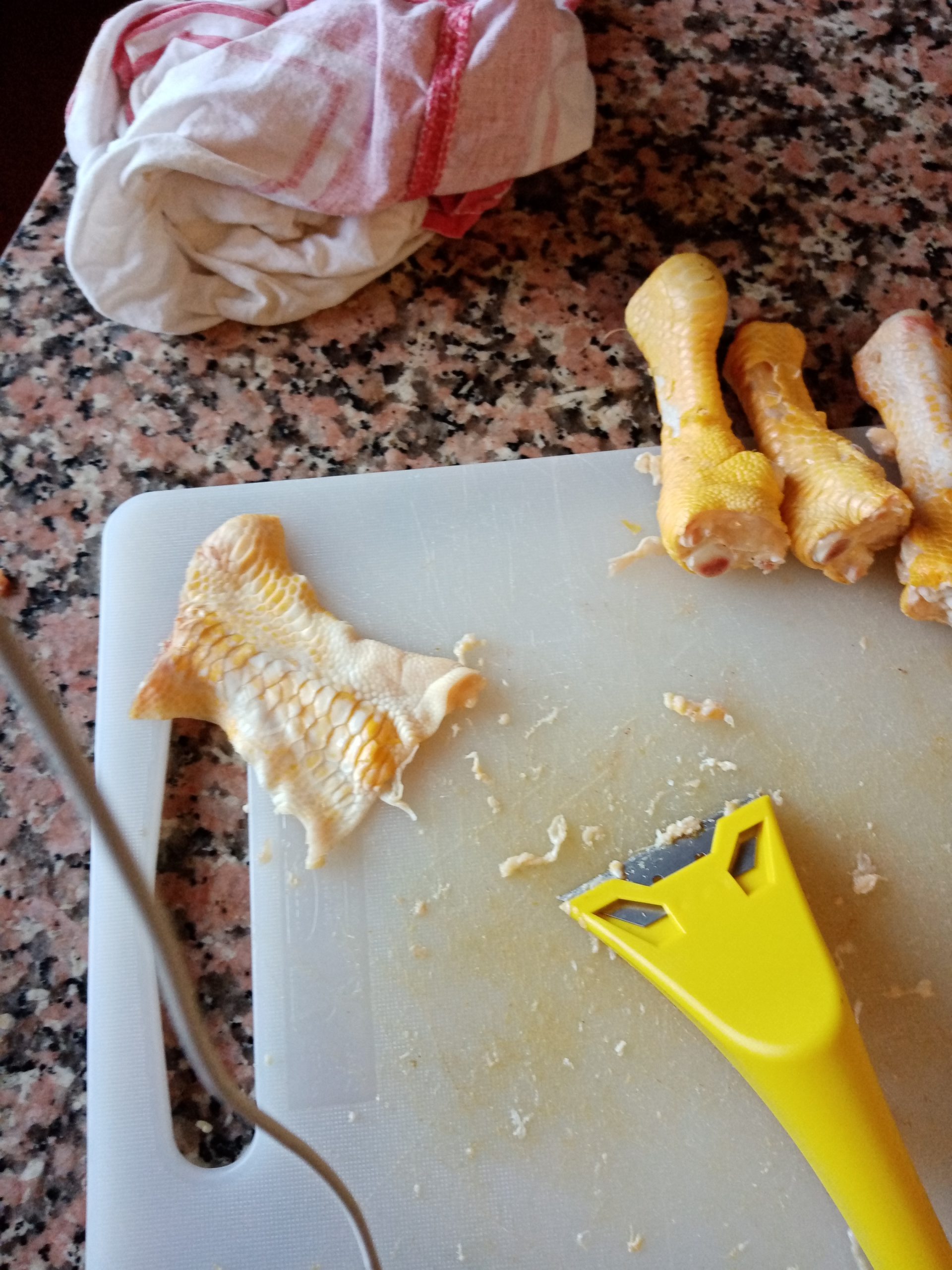
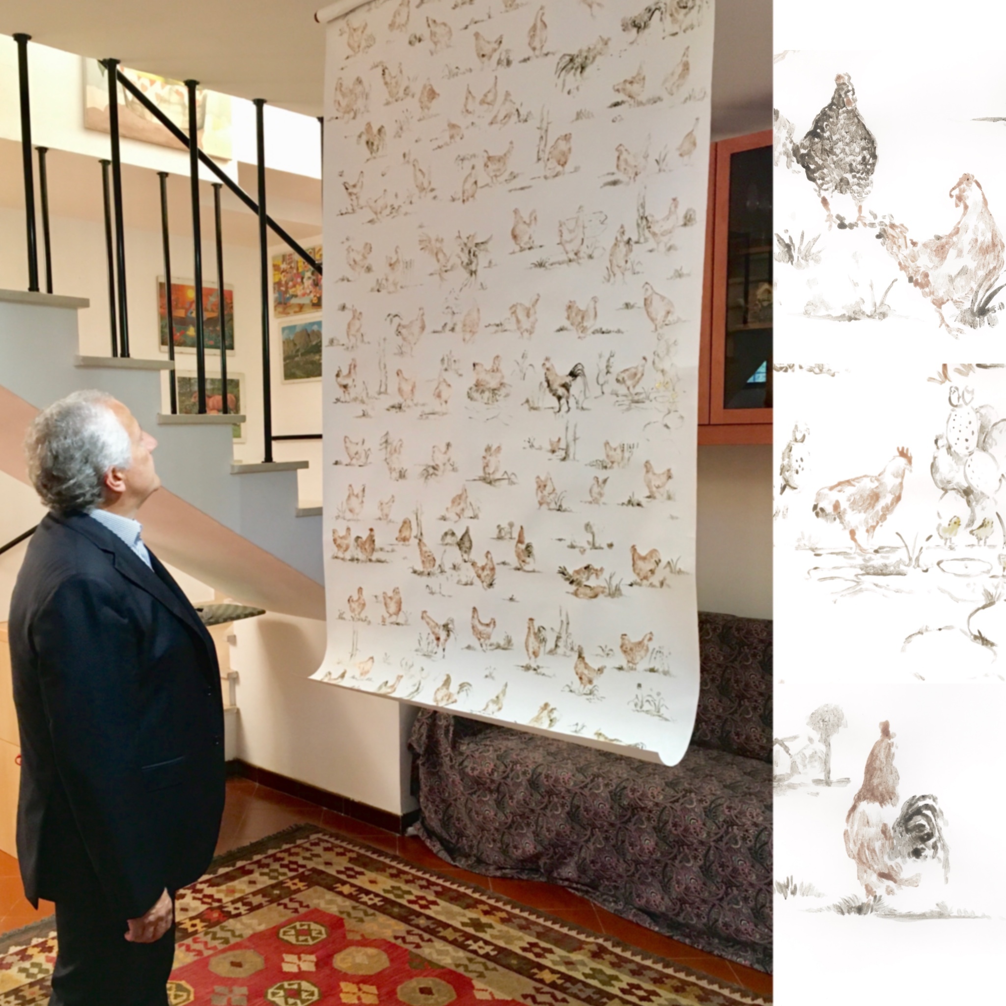
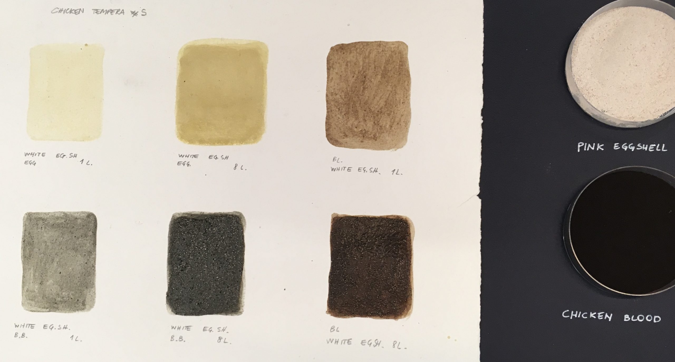
The chicken bone robot prototype I made turned out pretty well, mostly because bones have kind of gone through millions of years of evolution to be as strong and light as possible. Sounds like an ideal limb material. It’s also really nice to work with. Would be nice to do some composites too, for molding and 3D printing etc. from egg shells and feathers (2.3 million tonnes of EU feather waste from slaughterhouses a year) and whatever else.
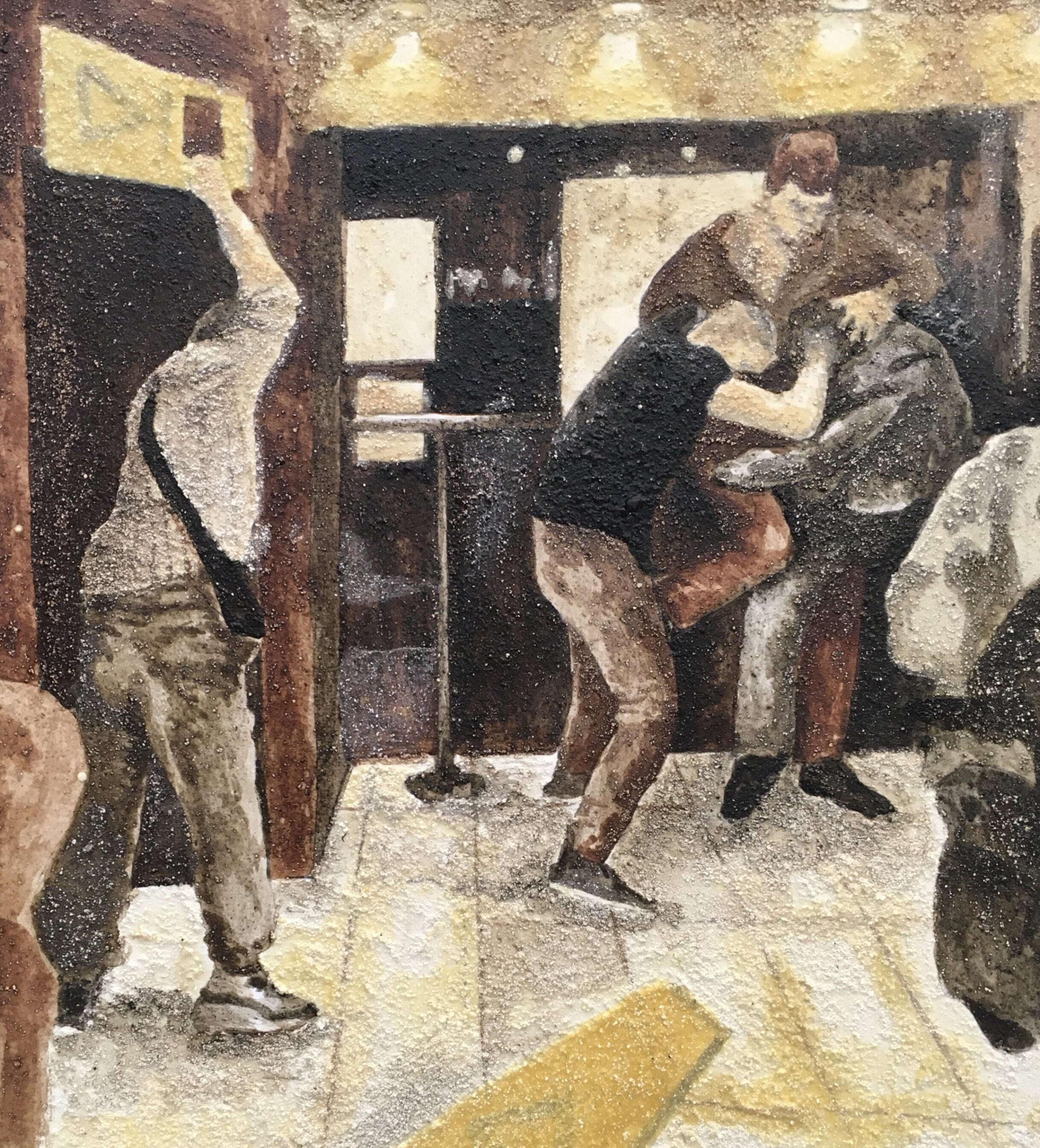
“Ecce” Robot pics from taken at the “making robots human ” exhibition in Stockholm Dan and I went to. The exhibition was kinda out of date British nationalist techno-utopian propaganda, but whatever, still got some cool hardware inspiration.


