After changing the normalisation code, (because the resampled 16000Hz audio was too soft), we have recordings from the microphone being classified by yamnet on the jetson.
Pretty cool. It’s detecting chicken sounds. I had to renormalize the recording volume between -1 and 1, as everything was originally detected as ‘Silence’.
Currently I’m saving 5 second wav files and processing them in Jupyter. But it’s not really interactive in a real-time way, and it would need further training to detect distress, or other, more useful metrics.
We’re unlikely to have time to implement the transfer learning, to continue with the chicken stress vocalisation work, for this project, but it definitely looks like the way to go about it.
There are also some papers that used the VGG-11 architecture for this purpose, chopping up recordings into overlapping 1 second segments, for training, matching them to a label (stressed / not stressed). Note: If downloading the dataset, use the G-Drive link, not the figshare link, which is truncated.
After following the installation procedure for my ‘Respeaker 2-Mic hat’, I’ve set up a dockerfile with TF2 and the audio libs, including librosa, in order to try out this real time version. Getting this right was a real pain, because of breaking changes in the ‘numba’ package.
FROM nvcr.io/nvidia/l4t-tensorflow:r32.6.1-tf2.5-py3

RUN apt-get update && apt-get install -y curl build-essential
RUN apt-get update && apt-get install -y libffi6 libffi-dev

RUN pip3 install -U Cython
RUN pip3 install -U pillow
RUN pip3 install -U numpy
RUN pip3 install -U scipy
RUN pip3 install -U matplotlib
RUN pip3 install -U PyWavelets
RUN pip3 install -U kiwisolver

RUN apt-get update && \
    apt-get install -y --no-install-recommends \
            alsa-base \
            libasound2-dev \
            alsa-utils \
            portaudio19-dev \
            libsndfile1 \
            unzip \
    && rm -rf /var/lib/apt/lists/* \
    && apt-get clean


RUN pip3 install soundfile pyaudio wave
RUN pip3 install tensorflow_hub
RUN pip3 install packaging
RUN pip3 install pyzmq==17.0.0
RUN pip3 install jupyterlab

RUN apt-get update && apt-get install -y libblas-dev \
				      liblapack-dev \
				      libatlas-base-dev \
				      gfortran \
				      protobuf-compiler \
				      libprotoc-dev \
		                      llvm-9 \
				      llvm-9-dev

RUN export LLVM_CONFIG=/usr/lib/llvm-9/bin/llvm-config && pip3 install llvmlite==0.36.0
RUN pip3 install --upgrade pip
RUN python3 -m pip install --user -U numba==0.53.1
RUN python3 -m pip install --user -U librosa==0.9.2
#otherwise matplotlib can't draw to gui
RUN apt-get update && apt-get install -y python3-tk


RUN jupyter lab --generate-config

RUN python3 -c "from notebook.auth.security import set_password; set_password('nvidia', '/root/.jupyter/jupyter_notebook_config.json')"

EXPOSE 6006
EXPOSE 8888

CMD /bin/bash -c "jupyter lab --ip 0.0.0.0 --port 8888 --allow-root &> /var/log/jupyter.log" & \
        echo "allow 10 sec for JupyterLab to start @ http://$(hostname -I | cut -d' ' -f1):8888 (password nvidia)" && \
        echo "JupterLab logging location:  /var/log/jupyter.log  (inside the container)" && \
        /bin/bash


I'm running it with

sudo docker run -it --rm --runtime nvidia --network host --privileged=true -e DISPLAY=$DISPLAY -v /tmp/.X11-unix:/tmp/.X11-unix -v /home/chicken/:/home/chicken nano_tf2_yamnet
NLP. Disambiguation: Not neurolinguistic programming, a discredited therapy, whereby one reprograms themselves, in a sense, to change their ill behaviours.
No, this one is about processing text. Sequence to sequence. Big models. Transformers. Just wondering now, if we need it. I saw an ad of some sort, for ‘Tagalog‘ and thought it was something about the Filipino language, but it was a product for NLP shops, for stuff like OCR, labelling, annotating, stuff. For mining text, basically.
Natural language processing is fascinating stuff, but probably out of the scope of this project. GPT-3 is the big one, and I think Google just released a network an order of magnitude bigger?
“Google’s new trillion-parameter AI language model is almost 6 times bigger than GPT-3”, so GPT-3 is old news anyway. I watched some interviews with the AI, and it’s very plucky. I can see why Elon is worried.
We’ve gone a totally different way, but this is another interesting project from Erwin Coumans, on the Google Brain team, who did PyBullet. NeuralSim replaces parts of physics engines with neural networks.
I just found this github from ETH Z. Not surprising that they have some of the most relevant datasets I’ve seen, pertaining to making proprioceptive autonomous systems. I came across their Autonomous Systems Labs dataset site.
One of the projects, panoptic mapping, is pretty much the panoptic segmentation from earlier research, combined with volumetric point clouds. “A flexible submap-based framework towards spatio-temporally consistent volumetric mapping and scene understanding.”
Here I’m continuing with the task of unsupervised detection of audio anomalies, hopefully for the purpose of detecting chicken stress vocalisations.
After much fussing around with the old Numenta NuPic codebase, I’m porting the older nupic.audio and nupic.critic code, over to the more recent htm.core.
These are the main parts:
Sparse Distributed Representation (SDR)
Encoders
Spatial Pooler (SP)
Temporal Memory (TM)
I’ve come across a very intricate implementation and documentation, about understanding the important parts in the HTM model, way deep, like how did I get here? I will try implement the ‘critic’ code, first. Or rather, I’ll try port it from nupic to htm. After further investigation, there’s a few options, and I’m going to try edit the hotgym example, and try shove wav files frequency band scalars through it instead of power consumption data. I’m simplifying the investigation. But I need to make some progress.
I’m using this docker to get in, mapping my code and wav file folder in:
docker run -d -p 8888:8888 --name jupyter -v /media/chrx/0FEC49A4317DA4DA/sounds/:/home/jovyan/work 3rdman/htm.core-jupyter:latest


So I've got some code working that writes to 'nupic format' (.csv) and code that reads the amplitudes from the csv file, and then runs it through htm.core.

So it takes a while, and it's just for 1 band (of 10 bands). I see it also uses the first 1/4 of so of the time to know what it's dealing with.  Probably need to run it through twice to get predictive results in the first 1/4.

Ok no, after a few weeks, I've come back to this point, and realise that the top graph is the important one.  Prediction is what's important.  The bottom graphs are the anomaly scores, used by the prediction.
Frequency Band 0
The idea in nupic.critic, was to threshold changes in X bands. Let’s see the other graphs…
Frequency band 0: 0-480Hz ?Frequency band 2: 960-1440Hz ?Frequency band 3: 1440-1920Hz ? Frequency band 4: 1920-2400Hz ? Frequency band 5: 2400-2880Hz ? Frequency band 6: 2880-3360Hz ?
Ok Frequency bands 7, 8, 9 were all zero amplitude. So that’s the highest the frequencies went. Just gotta check what those frequencies are, again…
Opening 307.wav
Sample width (bytes): 2
Frame rate (sampling frequency): 48000
Number of frames: 20771840
Signal length: 20771840
Seconds: 432
Dimensions of periodogram: 4801 x 2163

Ok with 10 buckets, 4801 would divide into
Frequency band 0: 0-480Hz
Frequency band 1: 480-960Hz
Frequency band 2: 960-1440Hz
Frequency band 3: 1440-1920Hz
Frequency band 4: 1920-2400Hz
Frequency band 5: 2400-2880Hz
Frequency band 6: 2880-3360Hz
Ok what else. We could try segment the audio by band, so we can narrow in on the relevant frequency range, and then maybe just focus on that smaller range, again, in higher detail.
Learning features with some labeled data, is probably the correct way to do chicken stress vocalisation detections.
Unsupervised anomaly detection might be totally off, in terms of what an anomaly is. It is probably best, to zoom in on the relevant bands and to demonstrate a minimal example of what a stressed chicken sounds like, vs a chilled chicken, and compare the spectrograms to see if there’s a tell-tale visualisable feature.
A score from 1 to 5 for example, is going to be anomalous in arbitrary ways, without labelled data. Maybe the chickens are usually stressed, and the anomalies are when they are unstressed, for example.
A change in timing in music might be defined, in some way. like 4 out of 7 bands exhibiting anomalous amplitudes. But that probably won’t help for this. It’s probably just going to come down to a very narrow band of interest. Possibly pointing it out on a spectrogram that’s zoomed in on the feature, and then feeding the htm with an encoding of that narrow band of relevant data.
I’ll continue here, with some notes on filtering. After much fuss, the sox app (apt-get install sox) does it, sort of. Still working on python version.
$ sox 307_0_50.wav filtered_50_0.wav sinc -n 32767 0-480
$ sox 307_0_50.wav filtered_50_1.wav sinc -n 32767 480-960
$ sox 307_0_50.wav filtered_50_2.wav sinc -n 32767 960-1440
$ sox 307_0_50.wav filtered_50_3.wav sinc -n 32767 1440-1920
$ sox 307_0_50.wav filtered_50_4.wav sinc -n 32767 1920-2400
$ sox 307_0_50.wav filtered_50_5.wav sinc -n 32767 2400-2880
$ sox 307_0_50.wav filtered_50_6.wav sinc -n 32767 2880-3360
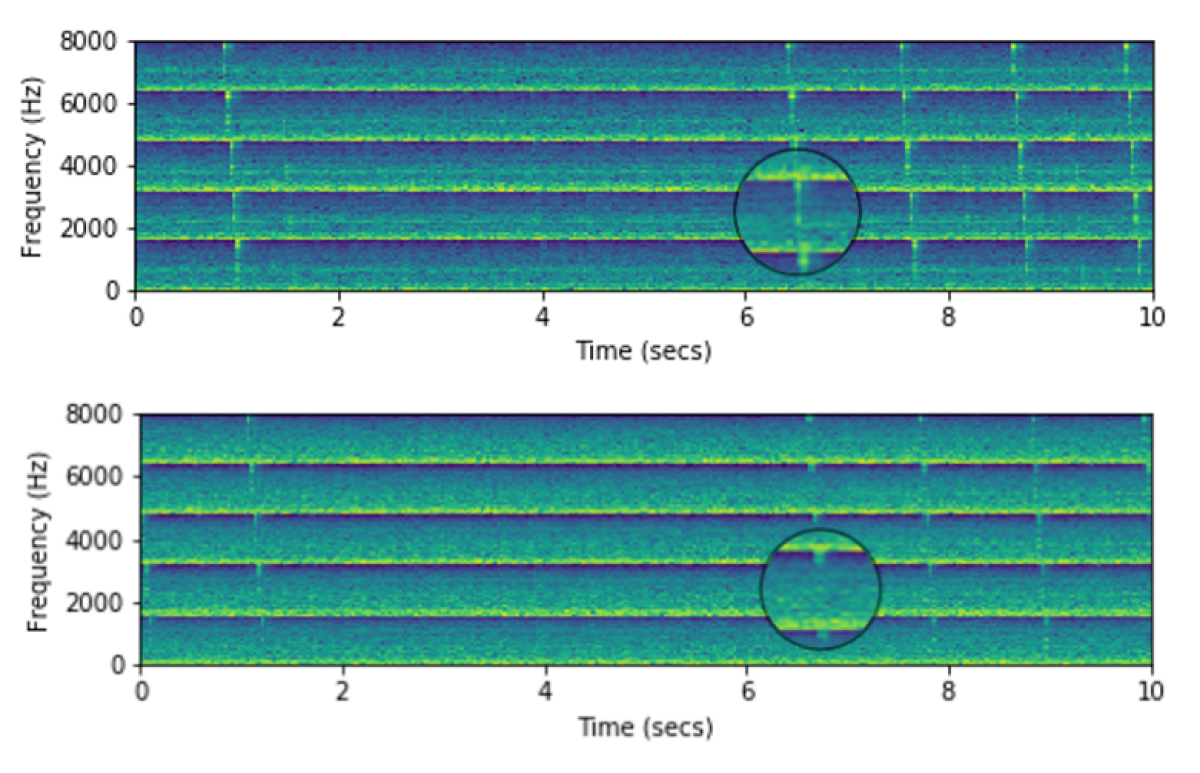
So, sox does seem to be working. The mel spectrogram is logarithmic, which is why it looks like this.
Visually, it looks like I'm interested in 2048 to 4096 Hz. That's where I can see the chirps.
Hmm. So I think the spectrogram is confusing everything.
So where does 4800 come from? 48 kHz. 48,000 Hz (48 kHz) is the sample rate “used for DVDs“.
Ah. Right. The spectrogram values represent buckets of 5 samples each, and the full range is to 24000…?
ok. So 2 x 24000. Maybe 2 channels? Anyway, full range is to 48000Hz. In that case, are the bands actually…
Frequency band 0: 0-4800Hz
Frequency band 1: 4800-9600Hz
Frequency band 2: 9600-14400Hz
Frequency band 3: 14400-19200Hz
Frequency band 4: 19200-24000Hz
Frequency band 5: 24000-28800Hz
Frequency band 6: 28800-33600Hz
Ok so no, it’s half the above because of the sample width of 2.
Frequency band 0: 0-2400Hz
Frequency band 1: 2400-4800Hz
Frequency band 2: 4800-7200Hz
Frequency band 3: 7200-9600Hz
Frequency band 4: 9600-12000Hz
Frequency band 5: 12000-14400Hz
Frequency band 6: 14400-16800Hz
So why is the spectrogram maxing at 8192Hz? Must be spectrogram sampling related.
So the original signal is 0 to 24000Hz, and the spectrogram must be 8192Hz because… the spectrogram is made some way. I’ll try get back to this when I understand it.
Ok i don’t entirely understand the last two. But basically the mel spectrogram is logarithmic, so those high frequencies really don’t get much love on the mel spectrogram graph. Buggy maybe.
So now I’m plotting the ‘chirp density’ (basically volume).
’98.wav’‘237.wav’‘307.wav’‘3072.wav’
In this scheme, we just proxy chirp volume density as a variable representing stress. We don’t know if it is a true proxy. As you can see, some recordings have more variation than others.
Some heuristic could be decided upon, for rating the stress from 1 to 5. The heuristic depends on how the program would be used. For example, if it were streaming audio, for an alert system, it might alert upon some duration of time spent above one standard deviation from the rolling mean. I’m not sure how the program would be used though.
If the goal were to differentiate stressed and not stressed vocalisations, that would require labelled audio data.
We’ve spoken with Dr. Maksimiljan Brus, at the University of Maribor, and he’s sent us some WAV file recordings of a large group of chickens.
There seems to be a decent amount of work done, particularly at Georgia Tech, regarding categorizing chicken sounds, to detect stress, or bronchitis, etc. They’ve also done some experiments to see how chickens react to humans and robots. (It takes them about 3 weeks to get used to either).
In researching the topic, there was a useful South African document related to smallholding size chicken businesses. It covers everything. Very good resource, actually, and puts into perspective the relative poverty in the communities where people sell chickens for a living. The profit margin per chicken in 2013 was about R12 per live chicken (less than 1 euro).
From PRODUCTION GUIDELINES for Small-Scale Broiler Enterprises K Ralivhesa, W van Averbeke & FK Siebrits
So anyway, I’m having a look at the sound files, to see what data and features I can extract. There’s no labels, so there won’t be any reinforcement learning here. Anomaly detection doesn’t need labels, and can use moving window statistics, to notice when something is out of the ordinary. So that’s what I’m looking into.
I am personally interested in Numenta’s algorithms, such as HTM, which use a model of cortical columns, and sparse encodings, to predict, and detect anomalies. I looked into getting Nupic.critic working, but Nupic is so old now, written in Python 2, that it’s practically impossible to get working. There is a community fork, htm.core, updated to Python 3, but it’s missing parts of the nupic codebase that nupic.critic is relying on. I’m able to convert the sound files to the nupic format, but am stuck for now, when running the analysis.
So let’s start at a more basic level and work our way up.
I downloaded Praat, an interesting sound analysis program used for some audio research. Not sure if it’s useful here. But it’s able to show various sound features. I’ll close it again, for now.
So, first thing to do, is going to be Mel spectrograms, and possibly Mel Frequency Cepstral Coefficients (MFCCs). The Mel scale kinda allows a difference between 250Hz and 500Hz to be scaled to the same size as a difference between 13250Hz and 13500Hz. It’s log-scaled.
Mel spectrograms let you use visual tools on audio. Also, worth knowing what a feature is, in machine learning. It’s a measurable property.
Ok where to start? Maybe librosa and PyOD?
pip install librosa
Ok and this outlier detection medium writeup, PyOD, says
Neural Networks
Neural networks can also be trained to identify anomalies.
Autoencoder (and variational autoencoder) network architectures can be trained to identify anomalies without labeled instances. Autoencoders learn to compress and reconstruct the information in data. Reconstruction errors are then used as anomaly scores.
More recently, several GAN architectures have been proposed for anomaly detection (e.g. MO_GAAL).
There’s also the results of a group working on this sort of problem, here.
Here was an illustrative example of an anomaly, of some machine sound.
And of course, there are more traditional? algorithms, (data-science algorithms). Here’s a medium article overview, for a submission to a heart murmur challenge. It mentions kapre, “Keras Audio Preprocessors – compute STFT, ISTFT, Melspectrogram, and others on GPU real-time.”
Here’s a useful flowchart from a paper about edge sound analysis on a Teensy. Smart Audio Sensors (SASs). The code “computes the FFT and Mel coefficients of a recorded audio frame.”
Smart Audio Sensors in the Internet of Things Edge for Anomaly Detection
I haven’t mentioned it, but of course FFT, Fast Fourier Transform, which converts audio to frequency bands, is going to be a useful tool, too. “The FFT’s importance derives from the fact that it has made working in the frequency domain equally computationally feasible as working in the temporal or spatial domain. ” – (wikipedia)
On the synthesis and possibly artistic end, there’s also MelGAN and the like.
Google’s got pipelines in kubernetes ? MLOps stuff.
Artistically speaking, it sounds like we want spectrograms. Someone implements one from scratch here, and there is a link to a good youtube video on relevant sound analysis ideas. Wide-band, vs. narrow-band, for example. Overlapping windows? They’re explaining STFT, which is used to make spectrograms.
Anyway. Good stuff. As always, I find the hardest part is finding your way back to your various dev environments. Ok I logged into the Jupyter running in the docker on the Jetson. ifconfig to get the ip, and http://192.168.101.115:8888/lab, voila).
Ok let’s see torchaudio’s colab… and pip install, ok… Here’s a summary of the colab.
Some ghostly Mel spectrogram stuff. Also, interesting ‘To recover a waveform from spectrogram, you can use GriffinLim.’
Ok let’s get our own dataset prepared. We need an anomaly detector. Let’s see…
———————— <LIBROSA INSTALLATION…> —————
Ok the librosa mel spectrogram is working, at least, so far. So these are the images for the 4 files Dr. Brus sent.
While looking for something like STFT to make a spectogram video, i came across this resource: Machine Hearing. Also this tome of ML resources.
Classification is maybe the best way to do this ML stuff. Then you can add labels to classes, and train a neural network to associate labels, and to categorise. So it would be ideal, if the data were pre-labelled, i.e. classified by chicken stress vocalisation experts. Like here is a soundset with metadata, that lets you classify sounds with labels, (with training).
So we really do need to use an anomaly detection algorithm, because I listened to the chickens for a little bit, and I’m not getting the nuances.
Here’s a relevant paper, which learns classes, for retroactive labelling. They’re recording a machine making sounds, and then humans label it. They say 1NN (k-nearest-neighbours) is hard to beat, but it’s memory intensive. “Nearest centroid (NC) combined with DBA has been shown to be competitive with kNN at a much smaller computational cost”.
Ok, let’s hope this old link works, for a nupic docker.
sudo docker run -i -t numenta/nupic /bin/bash
Ok amazing. Ok right, trying to install matplotlib inside the docker crashes. urllib3. I’ve been here before. Right, I asked on the github issues. 14 days ago, I asked. I got htm.core working. But it doesn’t have nupic.data classes.
After bashing my head against the apparent impossibility to pip install urllib3 and matplotlib in a python 2.7 docker, I’ve decided I will have to port the older nupic.critic or nupic.audio code to htm.core.
I cleared up some harddrive space, and ran this docker:
docker run -d -p 8888:8888 --name jupyter 3rdman/htm.core-jupyter:latest

then get the token for the URL:
docker logs -f jupyter
There’s a lot to go through, and I’m a noob at HTM. So I will start a new article now, on HTM specifically, for this.
I applied for the OpenAI Codex beta, and tried it out. It’s very cool.
It’s like GPT trained on Github or something like that, so you can just give it a prompt, and it tries to carry on the sentence with what it expects next.
So the easy way to use it, I’ve found, is to write a comment for the code you want it to write for you. I switched the engine to ‘davinci-codex’ and cranked up the response length to 1600 or so. Sometimes it just makes up more comments, or does something silly. But now and then it hits a home run.
Here’s an example.
"""
Take an example wav file, found at file_name="/home/jovyan/work/307.wav", and plot a mel spectrogram of it.
"""

import librosa
import librosa.display
import matplotlib.pyplot as plt

file_name="/home/jovyan/work/307.wav"

y, sr = librosa.load(file_name)

plt.figure(figsize=(12, 4))
librosa.display.waveplot(y, sr=sr)
plt.show()

S = librosa.feature.melspectrogram(y, sr=sr, n_mels=128)
log_S = librosa.power_to_db(S, ref=np.max)
plt.figure(figsize=(12, 4))
librosa.display.specshow(log_S, sr=sr, x_axis='time', y_axis='mel')
plt.title('mel power spectrogram')
plt.colorbar(format='%+02.0f dB')
plt.tight_layout()
plt.show()
I had to install librosa, but then it worked. It did more than I asked for.
Then I fed that whole thing, with another
"""
Plot the MFCC of file_name="/home/jovyan/work/307.wav"
"""
and it carried like an example giving champ:
"""
Take an example wav file, found at file_name="/home/jovyan/work/307.wav", and plot a mel spectrogram of it.
"""

import librosa
import librosa.display
import matplotlib.pyplot as plt

file_name="/home/jovyan/work/307.wav"

y, sr = librosa.load(file_name)

plt.figure(figsize=(12, 4))
librosa.display.waveplot(y, sr=sr)
plt.show()

S = librosa.feature.melspectrogram(y, sr=sr, n_mels=128)
log_S = librosa.power_to_db(S, ref=np.max)
plt.figure(figsize=(12, 4))
librosa.display.specshow(log_S, sr=sr, x_axis='time', y_axis='mel')
plt.title('mel power spectrogram')
plt.colorbar(format='%+02.0f dB')
plt.tight_layout()
plt.show()


"""
Plot the MFCC of file_name="/home/jovyan/work/307.wav"
"""

import librosa
import librosa.display
import matplotlib.pyplot as plt

file_name="/home/jovyan/work/307.wav"

y, sr = librosa.load(file_name)

plt.figure(figsize=(12, 4))
librosa.display.waveplot(y, sr=sr)
plt.show()

mfccs = librosa.feature.mfcc(y=y, sr=sr, n_mfcc=40)
plt.figure(figsize=(12, 4))
librosa.display.specshow(mfccs, x_axis='time')
plt.colorbar()
plt.title('MFCC')
plt.tight_layout()
plt.show()


"""
Plot the chromagram of file_name="/home/jovyan/work/307.wav"
"""

import librosa
import librosa.display
import matplotlib.pyplot as plt

file_name="/home/jovyan/work/307.wav"

y, sr = librosa.load(file_name)

plt.figure(figsize=(12, 4))
librosa.display.waveplot(y, sr=sr)
plt.show()

chroma = librosa.feature.chroma_stft(y=y, sr=sr)
plt.figure(figsize=(12, 4))
librosa.display.specshow(chroma, y_axis='chroma', x_axis='time')
plt.colorbar()
plt.title('Chromagram')
plt.tight_layout()
plt.show()


"""
Plot the tonnetz of file_name="/home/jovyan/work/307.wav"
"""

import librosa
import librosa.display
import matplotlib.pyplot as plt

file_name="/home/jovyan/work/307.wav"

y, sr = librosa.load(file_name)

plt.figure(figsize=(12, 4))
librosa.display.waveplot(y, sr=sr)
plt.show()

tonnetz = librosa.feature.tonnetz(y=y, sr=sr)
plt.figure(figsize=(12, 4))
librosa.display.specshow(tonnetz, y_axis='tonnetz', x_axis='time')
plt.colorbar()
plt.title('Tonal Centroids (Tonnetz)')
plt.tight_layout()
plt.show()


"""
Plot the zero-crossing rate of file_name="/home/jovyan/work/307.wav"
"""

import librosa
import librosa.display
import matplotlib.pyplot as plt

file_name="/home/jovyan/work/307.wav"

y, sr = librosa.load(file_name)

plt.figure(figsize=(12, 4))
librosa.display.waveplot(y, sr=sr)
plt.show()

zrate = librosa.feature.zero_crossing_rate(y)
plt.figure(figsize=(12, 4))
librosa.display.specshow(zrate, x_axis='time')
plt.colorbar()
plt.title('Zero Crossing Rate')
plt.tight_layout()
plt.show()


"""
Plot the spectral centroid of file_name="/home/jovyan/work/307.wav"
"""

import librosa
import librosa.display
import matplotlib.pyplot as plt

file_name="/home/jovyan/work/307.wav"

y, sr = librosa.load(file_name)

plt.figure(figsize=(12, 4))
librosa.display.waveplot(y, sr=sr)
plt.show()

cent = librosa.feature.spectral_centroid(y=y, sr=sr)
plt.figure(figsize=(12, 4))
librosa.display.specshow(cent, x_axis='time')
plt.colorbar()
plt.title('Spectral Centroids')
plt.tight_layout()
plt.show()


"""
Plot the spectral bandwidth of file_name="/home/jovyan/work/307.wav"
"""

import librosa
import librosa.display
import matplotlib.pyplot as plt

file_name="/home/jovyan/work/307.wav"

y, sr = librosa.load(file_name)

plt.figure(figsize=(12, 4))
librosa.display.waveplot(y, sr=sr)
plt.show()

spec_bw = librosa.feature.spectral_bandwidth(y=y, sr=sr)
plt.figure(figsize=(12, 4))
librosa.display.specshow(spec_bw, x_axis='time')
plt.colorbar()
plt.title('Spectral Bandwidth')
plt.tight_layout()
plt.show()


"""
Plot the spectral rolloff of file_name="/home/jovyan/work/307.wav"
"""

import librosa
import librosa.display
import matplotlib.pyplot as plt

file_name="/home/jovyan/work/307.wav"

y, sr = librosa.load(file_name)

plt.figure(figsize=(12, 4))
librosa.display.waveplot(y, sr=sr)
plt.show()

spec_rolloff = lib
After waiting a while… we get:
Ok, Chromagram twice… bold move, Codex.
import librosa
import librosa.display
import matplotlib.pyplot as plt

file_name="/home/jovyan/work/307.wav"

y, sr = librosa.load(file_name)

plt.figure(figsize=(12, 8))
D = librosa.amplitude_to_db(np.abs(librosa.stft(y)), ref=np.max)
plt.subplot(4, 2, 1)
librosa.display.specshow(D, y_axis='linear')
plt.colorbar(format='%+2.0f dB')
plt.title('Linear-frequency power spectrogram')

plt.subplot(4, 2, 2)
librosa.display.specshow(D, y_axis='log')
plt.colorbar(format='%+2.0f dB')
plt.title('Log-frequency power spectrogram')

plt.subplot(4, 2, 3)
librosa.display.specshow(D, x_axis='time')
plt.colorbar(format='%+2.0f dB')
plt.title('Time-frequency power spectrogram')

plt.subplot(4, 2, 4)
librosa.display.specshow(D, x_axis='time', y_axis='log')
plt.colorbar(format='%+2.0f dB')
plt.title('Log-Time-frequency power spectrogram')
Though I’m generally using stable baseline algorithms for training locomotion tasks, I am sometimes drawn back to evolutionary algorithms, and especially Map Elites, which has now been upgraded to incorporate a policy gradient.
The archiving of behaviours is what attracts me to Map Elites.
PGA Map Elites based on top of QDGym, which tracks Quality Diversity, is probably worth a look.
Beautiful. Since we’re currently just using a 256×256 view port in pybullet, this is quite a bit more advanced than required though. Learning game engines can also take a while. It took me about a month to learn Unity3d, with intermediate C# experience. Unreal Engine uses C++, so it’s a bit less accessible to beginners.