Finally tried shining light through an egg, and discovered calcium deposits making things opaque. Hmm.

This led to finding out about all these abnormal eggs.
Finally tried shining light through an egg, and discovered calcium deposits making things opaque. Hmm.
This led to finding out about all these abnormal eggs.
Here I’m continuing with the task of unsupervised detection of audio anomalies, hopefully for the purpose of detecting chicken stress vocalisations.
After much fussing around with the old Numenta NuPic codebase, I’m porting the older nupic.audio and nupic.critic code, over to the more recent htm.core.

These are the main parts:
I’ve come across a very intricate implementation and documentation, about understanding the important parts in the HTM model, way deep, like how did I get here? I will try implement the ‘critic’ code, first. Or rather, I’ll try port it from nupic to htm. After further investigation, there’s a few options, and I’m going to try edit the hotgym example, and try shove wav files frequency band scalars through it instead of power consumption data. I’m simplifying the investigation. But I need to make some progress.
I’m using this docker to get in, mapping my code and wav file folder in:
docker run -d -p 8888:8888 --name jupyter -v /media/chrx/0FEC49A4317DA4DA/sounds/:/home/jovyan/work 3rdman/htm.core-jupyter:latest


So I've got some code working that writes to 'nupic format' (.csv) and code that reads the amplitudes from the csv file, and then runs it through htm.core.

So it takes a while, and it's just for 1 band (of 10 bands). I see it also uses the first 1/4 of so of the time to know what it's dealing with.  Probably need to run it through twice to get predictive results in the first 1/4.

Ok no, after a few weeks, I've come back to this point, and realise that the top graph is the important one.  Prediction is what's important.  The bottom graphs are the anomaly scores, used by the prediction.

The idea in nupic.critic, was to threshold changes in X bands. Let’s see the other graphs…


Ok Frequency bands 7, 8, 9 were all zero amplitude. So that’s the highest the frequencies went. Just gotta check what those frequencies are, again…
Opening 307.wav
Sample width (bytes): 2
Frame rate (sampling frequency): 48000
Number of frames: 20771840
Signal length: 20771840
Seconds: 432
Dimensions of periodogram: 4801 x 2163

Ok with 10 buckets, 4801 would divide into
Frequency band 0: 0-480Hz
Frequency band 1: 480-960Hz
Frequency band 2: 960-1440Hz
Frequency band 3: 1440-1920Hz
Frequency band 4: 1920-2400Hz
Frequency band 5: 2400-2880Hz
Frequency band 6: 2880-3360Hz

Ok what else. We could try segment the audio by band, so we can narrow in on the relevant frequency range, and then maybe just focus on that smaller range, again, in higher detail.
Learning features with some labeled data, is probably the correct way to do chicken stress vocalisation detections.
Unsupervised anomaly detection might be totally off, in terms of what an anomaly is. It is probably best, to zoom in on the relevant bands and to demonstrate a minimal example of what a stressed chicken sounds like, vs a chilled chicken, and compare the spectrograms to see if there’s a tell-tale visualisable feature.
A score from 1 to 5 for example, is going to be anomalous in arbitrary ways, without labelled data. Maybe the chickens are usually stressed, and the anomalies are when they are unstressed, for example.
A change in timing in music might be defined, in some way. like 4 out of 7 bands exhibiting anomalous amplitudes. But that probably won’t help for this. It’s probably just going to come down to a very narrow band of interest. Possibly pointing it out on a spectrogram that’s zoomed in on the feature, and then feeding the htm with an encoding of that narrow band of relevant data.
I’ll continue here, with some notes on filtering. After much fuss, the sox app (apt-get install sox) does it, sort of. Still working on python version.
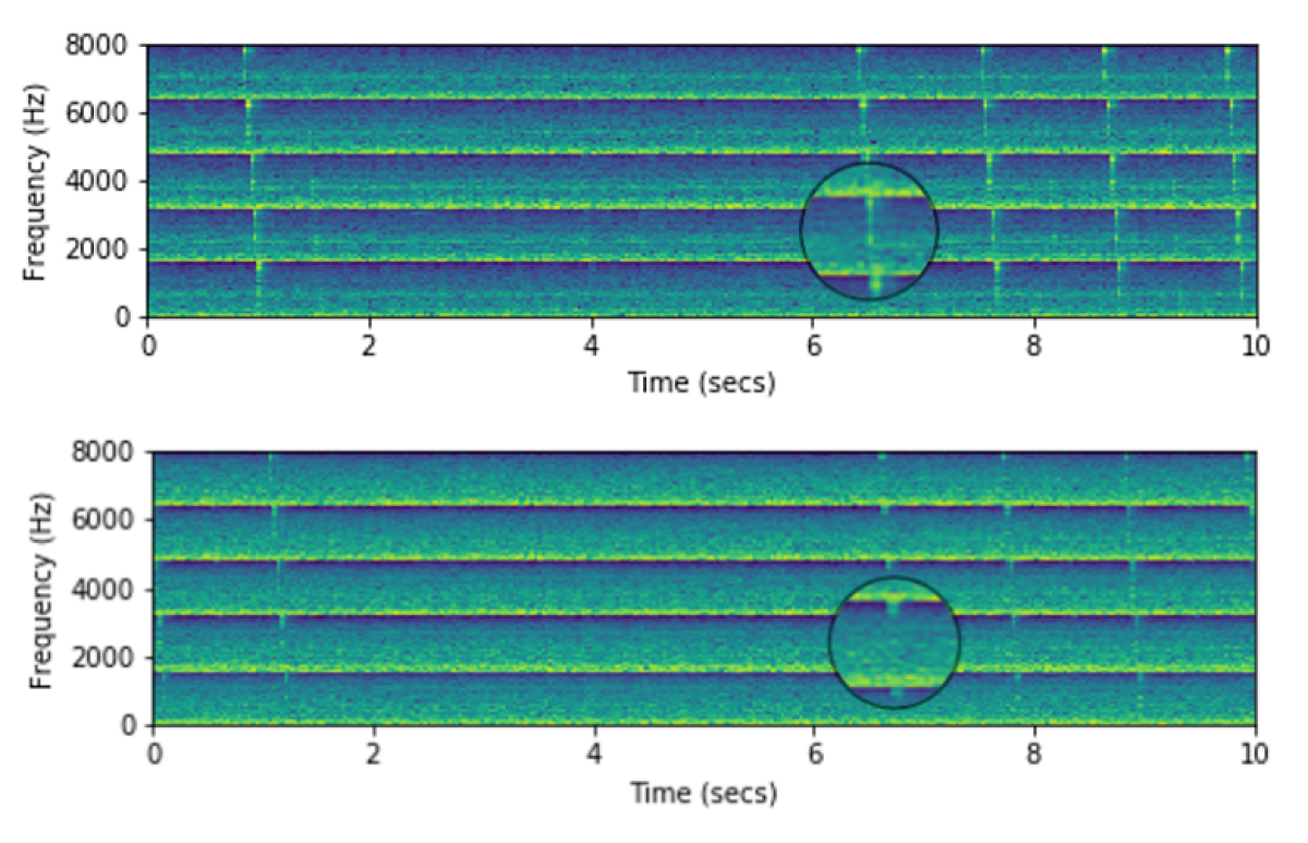
                                                                              $ sox 307_0_50.wav filtered_50_0.wav sinc -n 32767 0-480
$ sox 307_0_50.wav filtered_50_1.wav sinc -n 32767 480-960
$ sox 307_0_50.wav filtered_50_2.wav sinc -n 32767 960-1440
$ sox 307_0_50.wav filtered_50_3.wav sinc -n 32767 1440-1920
$ sox 307_0_50.wav filtered_50_4.wav sinc -n 32767 1920-2400
$ sox 307_0_50.wav filtered_50_5.wav sinc -n 32767 2400-2880
$ sox 307_0_50.wav filtered_50_6.wav sinc -n 32767 2880-3360


So, sox does seem to be working.  The mel spectrogram is logarithmic, which is why it looks like this.

Visually, it looks like I'm interested in 2048 to 4096 Hz.  That's where I can see the chirps.

Hmm. So I think the spectrogram is confusing everything.
So where does 4800 come from? 48 kHz. 48,000 Hz (48 kHz) is the sample rate “used for DVDs“.
Ah. Right. The spectrogram values represent buckets of 5 samples each, and the full range is to 24000…?
Sample width (bytes): 2
0.     5.    10.    15.    20.    25.    30.    35.    40.    45.    50.    55.    60.    65.    70.    75.    80.    85.    90.    95.    100.   105.   110.   115.   120.   125.   130.   135.   140.   145.
...
 23950. 23955. 23960. 23965. 23970. 23975. 23980. 23985. 23990. 23995. 24000.]
ok. So 2 x 24000. Maybe 2 channels? Anyway, full range is to 48000Hz. In that case, are the bands actually…
Frequency band 0: 0-4800Hz
Frequency band 1: 4800-9600Hz
Frequency band 2: 9600-14400Hz
Frequency band 3: 14400-19200Hz
Frequency band 4: 19200-24000Hz
Frequency band 5: 24000-28800Hz
Frequency band 6: 28800-33600Hz
Ok so no, it’s half the above because of the sample width of 2.
Frequency band 0: 0-2400Hz
Frequency band 1: 2400-4800Hz
Frequency band 2: 4800-7200Hz
Frequency band 3: 7200-9600Hz
Frequency band 4: 9600-12000Hz
Frequency band 5: 12000-14400Hz
Frequency band 6: 14400-16800Hz
So why is the spectrogram maxing at 8192Hz? Must be spectrogram sampling related.

So the original signal is 0 to 24000Hz, and the spectrogram must be 8192Hz because… the spectrogram is made some way. I’ll try get back to this when I understand it.
sox 307_0_50.wav filtered_50_0.wav sinc -n 32767 0-2400
sox 307_0_50.wav filtered_50_1.wav sinc -n 32767 2400-4800
sox 307_0_50.wav filtered_50_2.wav sinc -n 32767 4800-7200
sox 307_0_50.wav filtered_50_3.wav sinc -n 32767 7200-9600
sox 307_0_50.wav filtered_50_4.wav sinc -n 32767 9600-12000
sox 307_0_50.wav filtered_50_5.wav sinc -n 32767 12000-14400
sox 307_0_50.wav filtered_50_6.wav sinc -n 32767 14400-16800

Ok I get it now.


Ok i don’t entirely understand the last two. But basically the mel spectrogram is logarithmic, so those high frequencies really don’t get much love on the mel spectrogram graph. Buggy maybe.
But I can estimate now the chirp frequencies…
sox 307_0_50.wav filtered_bird.wav sinc -n 32767 1800-5200

Beautiful. So, now to ‘extract the features’…
So, the nupic.critic code with 1 bucket managed to get something resembling the spectrogram. Ignore the blue.
But it looks like maybe, we can even just threshold and count peaks. That might be it.

sox 307.wav filtered_307.wav sinc -n 32767 1800-5200
sox 3072.wav filtered_3072.wav sinc -n 32767 1800-5200
sox 237.wav filtered_237.wav sinc -n 32767 1800-5200
sox 98.wav filtered_98.wav sinc -n 32767 1800-5200
Let’s do the big files…

Ok looks good enough.
So now I’m plotting the ‘chirp density’ (basically volume).


In this scheme, we just proxy chirp volume density as a variable representing stress. We don’t know if it is a true proxy.
As you can see, some recordings have more variation than others.
Some heuristic could be decided upon, for rating the stress from 1 to 5. The heuristic depends on how the program would be used. For example, if it were streaming audio, for an alert system, it might alert upon some duration of time spent above one standard deviation from the rolling mean. I’m not sure how the program would be used though.
If the goal were to differentiate stressed and not stressed vocalisations, that would require labelled audio data.
(Also, basically didn’t end up using HTM, lol)
We’ve spoken with Dr. Maksimiljan Brus, at the University of Maribor, and he’s sent us some WAV file recordings of a large group of chickens.
There seems to be a decent amount of work done, particularly at Georgia Tech, regarding categorizing chicken sounds, to detect stress, or bronchitis, etc. They’ve also done some experiments to see how chickens react to humans and robots. (It takes them about 3 weeks to get used to either).
In researching the topic, there was a useful South African document related to smallholding size chicken businesses. It covers everything. Very good resource, actually, and puts into perspective the relative poverty in the communities where people sell chickens for a living. The profit margin per chicken in 2013 was about R12 per live chicken (less than 1 euro).

So anyway, I’m having a look at the sound files, to see what data and features I can extract. There’s no labels, so there won’t be any reinforcement learning here. Anomaly detection doesn’t need labels, and can use moving window statistics, to notice when something is out of the ordinary. So that’s what I’m looking into.
I am personally interested in Numenta’s algorithms, such as HTM, which use a model of cortical columns, and sparse encodings, to predict, and detect anomalies. I looked into getting Nupic.critic working, but Nupic is so old now, written in Python 2, that it’s practically impossible to get working. There is a community fork, htm.core, updated to Python 3, but it’s missing parts of the nupic codebase that nupic.critic is relying on. I’m able to convert the sound files to the nupic format, but am stuck for now, when running the analysis.
So let’s start at a more basic level and work our way up.
I downloaded Praat, an interesting sound analysis program used for some audio research. Not sure if it’s useful here. But it’s able to show various sound features. I’ll close it again, for now.

So, first thing to do, is going to be Mel spectrograms, and possibly Mel Frequency Cepstral Coefficients (MFCCs). The Mel scale kinda allows a difference between 250Hz and 500Hz to be scaled to the same size as a difference between 13250Hz and 13500Hz. It’s log-scaled.
Mel spectrograms let you use visual tools on audio. Also, worth knowing what a feature is, in machine learning. It’s a measurable property.
Ok where to start? Maybe librosa and PyOD?
pip install librosa
Ok and this outlier detection medium writeup, PyOD, says
Neural networks can also be trained to identify anomalies.
Autoencoder (and variational autoencoder) network architectures can be trained to identify anomalies without labeled instances. Autoencoders learn to compress and reconstruct the information in data. Reconstruction errors are then used as anomaly scores.
More recently, several GAN architectures have been proposed for anomaly detection (e.g. MO_GAAL).
There’s also the results of a group working on this sort of problem, here.
A relevant arxiv too:
ANOMALOUS SOUND DETECTION BASED ON
INTERPOLATION DEEP NEURAL NETWORK
And
UNSUPERVISED ANOMALOUS SOUND DETECTION VIA AUTOENCODER APPROACH
What is this DCASE?
Hmm so there is a challenge for it currently. It’s big in Japan. Here’s the winning solution:
Amazon programmers win an Amazon competition on anomaly detection.
Here was an illustrative example of an anomaly, of some machine sound.
And of course, there are more traditional? algorithms, (data-science algorithms). Here’s a medium article overview, for a submission to a heart murmur challenge. It mentions kapre, “Keras Audio Preprocessors – compute STFT, ISTFT, Melspectrogram, and others on GPU real-time.”
And I found ‘torchaudio‘,
Here’s a useful flowchart from a paper about edge sound analysis on a Teensy. Smart Audio Sensors (SASs). The code “computes the FFT and Mel coefficients of a recorded audio frame.”

I haven’t mentioned it, but of course FFT, Fast Fourier Transform, which converts audio to frequency bands, is going to be a useful tool, too. “The FFT’s importance derives from the fact that it has made working in the frequency domain equally computationally feasible as working in the temporal or spatial domain. ” – (wikipedia)
On the synthesis and possibly artistic end, there’s also MelGAN and the like.
Google’s got pipelines in kubernetes ? MLOps stuff.
Artistically speaking, it sounds like we want spectrograms. Someone implements one from scratch here, and there is a link to a good youtube video on relevant sound analysis ideas. Wide-band, vs. narrow-band, for example. Overlapping windows? They’re explaining STFT, which is used to make spectrograms.
There’s also something called Chirp Z transform.
Anyway. Good stuff. As always, I find the hardest part is finding your way back to your various dev environments. Ok I logged into the Jupyter running in the docker on the Jetson. ifconfig to get the ip, and http://192.168.101.115:8888/lab, voila).
Ok let’s see torchaudio’s colab… and pip install, ok… Here’s a summary of the colab.
Some ghostly Mel spectrogram stuff. Also, interesting ‘To recover a waveform from spectrogram, you can use GriffinLim.’

Ok let’s get our own dataset prepared. We need an anomaly detector. Let’s see…
———————— <LIBROSA INSTALLATION…> —————
Ok the librosa mel spectrogram is working, at least, so far. So these are the images for the 4 files Dr. Brus sent.

While looking for something like STFT to make a spectogram video, i came across this resource: Machine Hearing. Also this tome of ML resources.
Classification is maybe the best way to do this ML stuff. Then you can add labels to classes, and train a neural network to associate labels, and to categorise. So it would be ideal, if the data were pre-labelled, i.e. classified by chicken stress vocalisation experts. Like here is a soundset with metadata, that lets you classify sounds with labels, (with training).
So we really do need to use an anomaly detection algorithm, because I listened to the chickens for a little bit, and I’m not getting the nuances.
Here’s a relevant paper, which learns classes, for retroactive labelling. They’re recording a machine making sounds, and then humans label it. They say 1NN (k-nearest-neighbours) is hard to beat, but it’s memory intensive. “Nearest centroid (NC) combined with DBA has been shown to be competitive with kNN at a much smaller computational cost”.
Here’s pyAudioAnalysis
Perform unsupervised segmentation (e.g. speaker diarization) and extract audio thumbnails
Here’s a cool visualiser, in tensorboard,

Ideally, I would like to use NuPIC.
Ok, let’s hope this old link works, for a nupic docker.
sudo docker run -i -t numenta/nupic /bin/bash
Ok amazing. Ok right, trying to install matplotlib inside the docker crashes. urllib3. I’ve been here before. Right, I asked on the github issues. 14 days ago, I asked. I got htm.core working. But it doesn’t have nupic.data classes.
After bashing my head against the apparent impossibility to pip install urllib3 and matplotlib in a python 2.7 docker, I’ve decided I will have to port the older nupic.critic or nupic.audio code to htm.core.
I cleared up some harddrive space, and ran this docker:
docker run -d -p 8888:8888 --name jupyter 3rdman/htm.core-jupyter:latest

then get the token for the URL:
docker logs -f jupyter
There’s a lot to go through, and I’m a noob at HTM. So I will start a new article now, on HTM specifically, for this.
“They observed that many quadrupedal, mammalian animals feature a distinguished functional three-segment front leg and hind leg design, and proposed a “pantograph” leg abstraction for robotic research.”
1 DOF (degree of freedom). 1 motor. Miranda wants jointed legs, and I don’t want to work out inverse kinematics, so this looks ideal. Maybe a bit complicated still.

The simpler force diagram:

 Kinematic primitives for walking and trotting gaits of a quadruped robot with compliant legs (Alexander Badri-Spröwitz et al, 2014)
Compliance is a feature, made possible by springs typically.

A homemade attempt here with the Mojo robot of the Totally Not Evil Robot Army. Their robot only uses 9g servos, and can’t quite pick itself up.
I did an initial design with what I had around, and it turns out compliance is a delicate balance. Too much spring, and it just mangles itself up. Too little spring and it can’t lift off the ground.
Further iterations removed the springs, which were too tight by far, and used cable ties to straighten the legs, but the weight of the robot is a little bit too much for the knee joints.
I will likely leave it until I have a 3d printer, some better springs, and will give it another try with more tools and materials available. Maybe even hydraulics, some day,
Some more research required, too.
Lot’s of interesting stuff.
Fighting: “This fighting often continues until they reach maturity and the pecking order is well established.”
Foraging: “In the wild, jungle fowl spend 61% of their time foraging. Foraging behaviors include pecking and scratching at potential food sources, as well as looking for and sampling possible food sources. Providing chickens with a complete feed eliminates the need for foraging in order to obtain nutrients, but the hens will continue performing this behavior”
Nesting: “Birds are mimics”
Ethology lecture, Sapolsky: https://www.youtube.com/watch?v=ISVaoLlW104
Possibly very interesting… Neuroethology: https://en.wikipedia.org/wiki/Neuroethology
Also, neurorobotics: